Three-dimensional aerosols are obtained for individual species from the GEOS-Chem model. This helps provide information on aerosol optical depth (AOD) and surface visibility. For SWIm a size distribution and phase function are computed for each aerosol species. The resultant phase function along each line of sight is given by a linear combination of the fractional contribution of each species present in the analysis in the vicinity of the ray path.
There is an option to utilize HRRR-Smoke and PM2.5 data to locally increase the smoke aerosols from wildfires if they aren't fully resolved by GEOS-Chem.
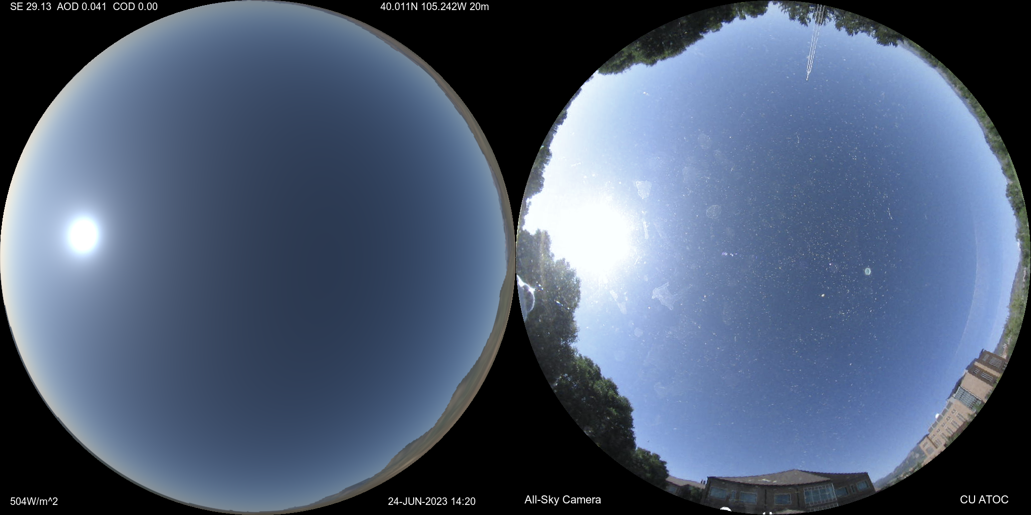
This comparison of simulated and camera images at the University of Colorado Sky Observatory in Boulder shows good correlation in patterns of brightness throughout the sky. The variations are caused by different path lengths through the atmosphere, and the variation of scattering by air molecules and aerosols at different angular distances from the sun.
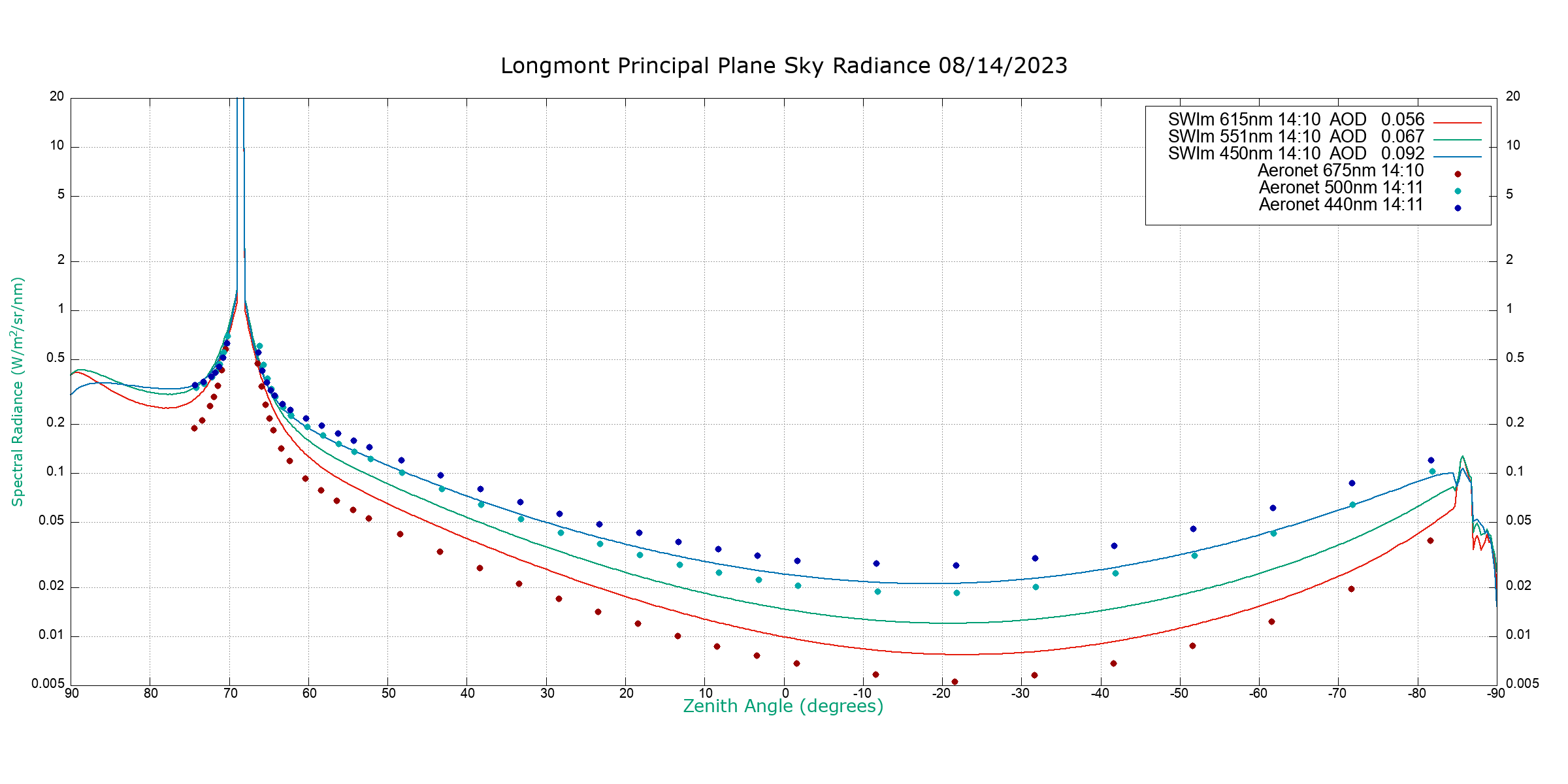
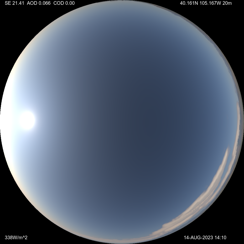
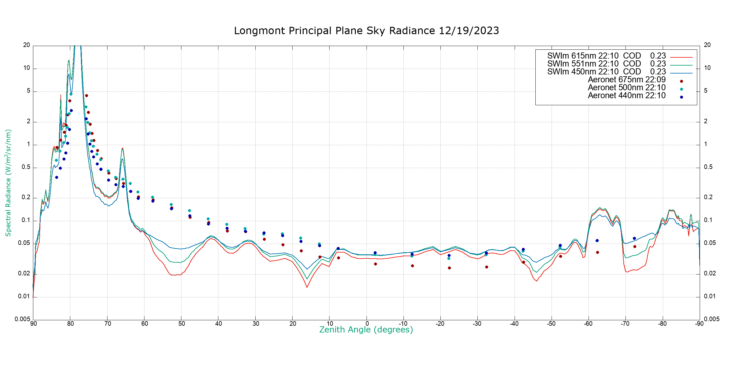
Aeronet validation is shown above using simulated and observed multi-spectral sky radiances along the principal plane. This is a mostly cloud-free case with the sun in the eastern sky on August 14, 2023 as seen from Longmont, Colorado. The solid lines show simulated sky brightness (spectral radiance) at three wavelengths, on the principal plane passing vertically through the sun. A zenith angle of -90 is on the horizon below the sun, 0 denotes the zenith, and +90 is on anti-solar horizon. The circles represent spectral radiance measurements from Aeronet at three roughly similar wavelengths. The observed wavelengths differ somewhat from the simulated values contributring to a vertical offset. The curves tend to peak near the sun's location due to forward scattering light from aerosols.
Near the zenith we are looking mostly at a deeper blue sky from Rayleigh scattering. Here the blue lines representing SWIm radiances should be positioned close to the blue Aeronet dots since they are only 10nm apart in wavelength, just slightly lower on the logarithmic plot separated by a ratio of 1.094. Generally the calculated 450nm radiance at the zenith is about 5-15% lower than expected. The overall shape of the brightness profile throughout the principal plane looks good. The bright high radiance values in the forward scattering peak area near the sun are strongly influenced by aerosols. Some refinements are being tested to help show more of a crossover between the SWIm blue and green lines as we climb towards the peak, just as the corresponding Aeronet radiances do.
This is a clear sky case with approximately 30% proportion of dust from the GEOS-Chem model. A case with more smoke will be anticipated to have a smaller dust proportion in GOES-Chem and more Organic Carbon and Sulfates. These phase functions have a less pronounced forward scattering peak near the sun.
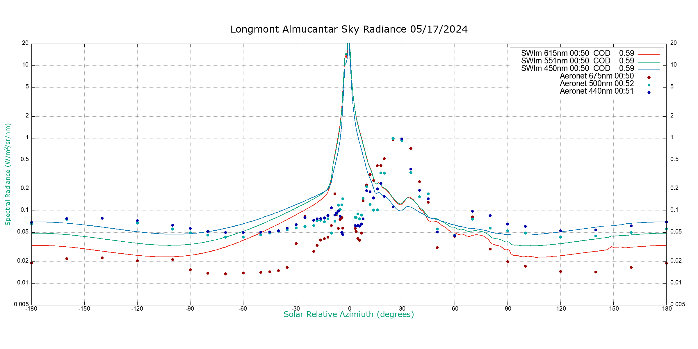
Here are the latest near-realtime comparisons of
almucantar radiance (sky brightness)
,
principal plane radiance (sky brightness)
at several wavelengths, and
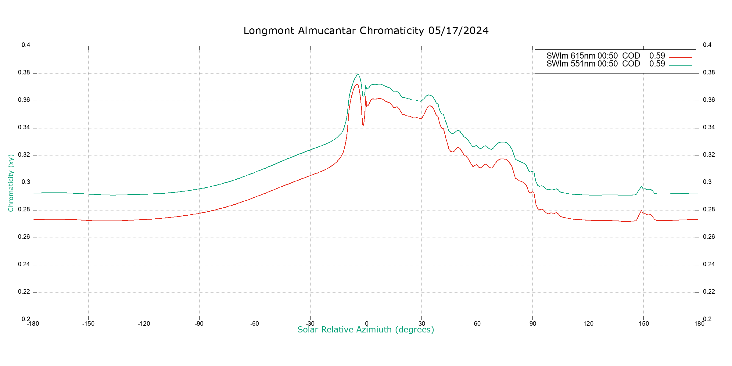
chromaticity (sky color)
.
The almucantar is a circle around the sky passing through the sun at constant elevation angle, where the x-axis represents azimuth difference compared with the solar azimuth.
In the chromaticity plot, the red line is the "x" value and the green line is the "y" value. Lower values represent bluer colors and higher values
trend more towards white, or even reddish at the top of the scale.
These plots often represent a combination of sky regions having various amounts of cloud cover. Simpler cases will be all-clear or all-cloudy.
The type of case can be assessed by checking nearby
all-sky cameras
from the region at the plot comparison time.
Thanks to Janae Csavina from NEON/Battelle in Longmont for the
Aeronet radiance observations
.
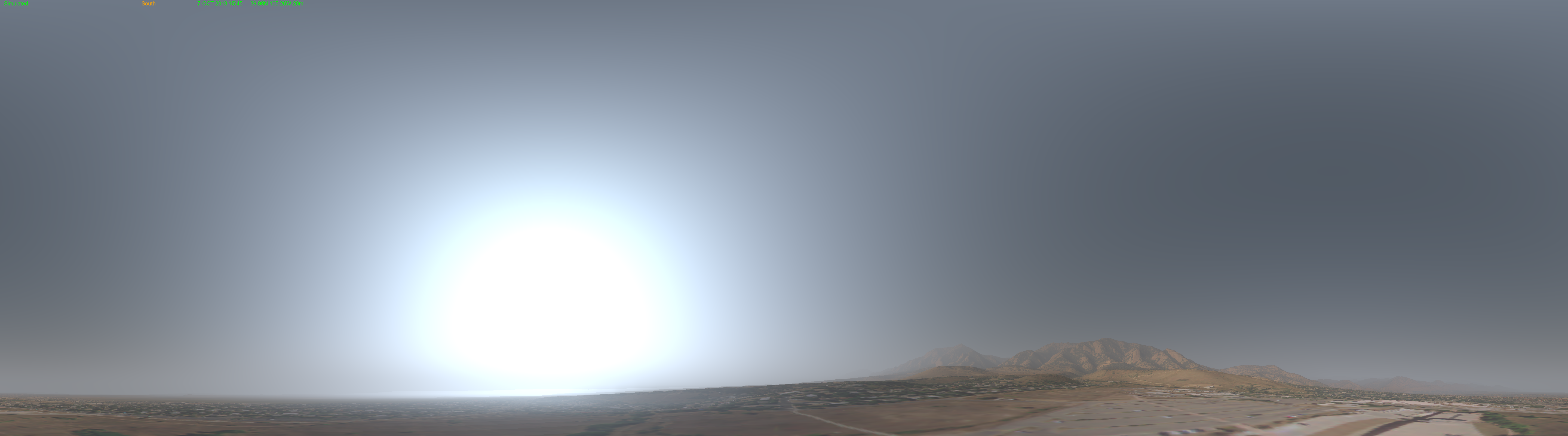
A simulated landscape and sky from Boulder Colorado is shown above using an idealized aerosol field. The ray-tracing utilizes a
30m horizontal grid, 1/16 degree angular resolution with land imagery from USDA and Descartes.
Here is a
virtual reality version
of a clearer sky view
and a series of frames with various amounts of
smoke aerosols added
.
Each frame has a differing amount of aerosols, characterized by parameters such as aerosol optical depth (AOD) and scale height representing the vertical profile,
to specify a 3-dimensional field of aerosol extinction coefficient (AEC).
Surface visibility, more formally known as meteorological optical range, can be determined by knowing the AEC at the surface.
In this
large format animation
one can roam around to look in various directions.
It's interesting to look to the west and see the Flatirons near Boulder become more obscured, while the sun turns red to the southeast.
Visibility Reduction
Visibility Analysis
A
real-time look
at visibility is shown above using the Colorado analysis fields. A recorded AMS video presentation on general aspects of visibility and the sky simulations can be
viewed here
.
