LAPS Cloud Downscaling Algorithm
1. Algorithm Overview
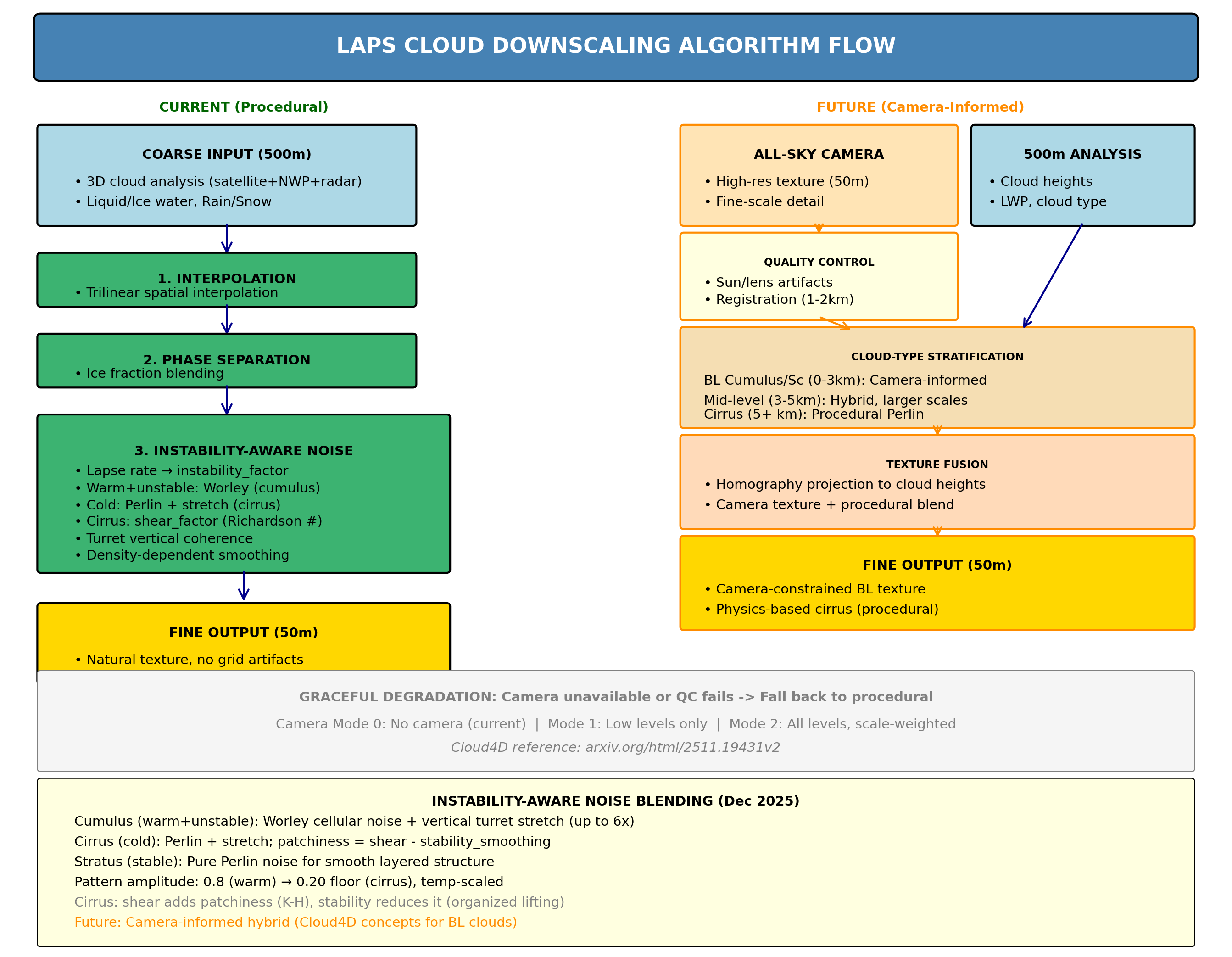
The LAPS (Local Analysis and Prediction System) cloud downscaling algorithm converts coarse-resolution cloud data into high-resolution fields using stability-aware Perlin/Worley noise blending. The algorithm combines trilinear interpolation with physics-based noise generation applied at global fine grid coordinates to create realistic fine-scale cloud structures without grid artifacts.
Current Design (December 2025): The implementation uses atmospheric stability and temperature to dynamically blend between Worley noise (cellular cumulus patterns) and Perlin noise (smooth stratus/cirrus patterns). Warm, unstable air triggers cumulus-appropriate Worley cellular structures with vertically elongated turrets, while cold or stable air produces smooth Perlin patterns with anisotropic stretching for cirrus. All transitions are continuous to prevent artifacts. Anti-mottling provides density-dependent smoothing in dense cloud regions while preserving natural texture in lighter areas.
1.1 Key Characteristics
- Stability-Aware: Lapse rate determines convective instability → Worley weight
- Temperature-Aware: Warm cloud factor limits cumulus treatment to boundary layer
- Continuous Transitions: All parameters blend smoothly to prevent artifacts
- Cloud-Type Appropriate: Worley for cumulus, Perlin for stratus, stretched Perlin for cirrus
- Vertical Coherence: Dynamic turret structure (2-8x stretch) for realistic cumulus towers
- Real-time Operational: Efficient computation suitable for operational NWP systems
Figure 1: Cloud Downscaling Algorithm Flowchart
2. Core Algorithm Steps
2.1 Trilinear Interpolation
Standard trilinear spatial interpolation creates the initial fine-grid field from coarse-grid data, providing smooth base values across the domain while preserving the input data structure.
2.2 Direct Pattern Generation + Modulation Reduction
Core Innovation: Generate Perlin/Worley patterns directly at global fine grid coordinates during final processing. For each fine grid point, call atmospheric turbulence generation using global position coordinates, then apply density-dependent modulation reduction smoothing.
2.3 Tunable Parameters
pattern_amplitude: Controls clearing intensity (default 1.0, reduce to ~0.9 for smaller clearings).
blend_strength: Controls modulation reduction intensity (0.7 = 70% smoothing in dense areas).
density_center/width: Controls density thresholds for modulation reduction transitions.
3. Current Implementation (December 2025)
3.1 Instability-Aware Perlin/Worley Noise Blending
The current implementation uses instability-aware Perlin/Worley noise blending that adapts to atmospheric conditions. This approach generates appropriate patterns for different cloud types: cellular Worley patterns for unstable cumulus, smooth Perlin for stable stratus, and anisotropically-stretched Perlin for cold cirrus with Richardson number-based patchiness for jet stream cirrus.
Instability Factor Calculation (updated Jan 2026)
- Lapse Rate: Calculated from vertical temperature gradient (K/km)
- Neutral Lapse Rate: Temperature-dependent via
get_neutral_lapse_rate()— approximates MALR behavior (warm ~5 K/km, cold ~8 K/km) - instability_factor: 0.0 at neutral → 1.0 at neutral + 4 K/km (approaching dry adiabatic)
- Formula:
instability_factor = clamp((lapse_rate - neutral_lapse_rate) / 4.0, 0.0, 1.0) - Consistency: Now uses same temperature-dependent threshold as stability-based smoothing (Section 3.4)
Warm Cloud Factor
- Purpose: Limits cumulus treatment to boundary layer air (warm, moist convection)
- Range: 1.0 at 290K (17°C) → 0.0 at 253K (-20°C)
- Effect: Cold air (cirrus regime) uses cirrus-specific physics instead
Effective Instability & Worley Blending
- effective_instability:
instability_factor × warm_cloud_factor × cirrus_damping - worley_weight:
effective_instability × 0.5(up to 50% Worley for strong cumulus) - Perlin weight:
1.0 - worley_weight(always blended, never step change)
Dynamic Vertical Correlation
- Base: 2.0 (standard vertical correlation)
- Instability boost: +4.0 × effective_instability (taller cells for cumulus turrets)
- Temperature boost: +2.0 × temp_factor (enhanced for cold cirrus)
- Result: 2.0-8.0 range creates appropriate vertical structure for each cloud type
3.2 Cirrus Richardson Number Physics
For cirrus clouds, the Richardson number (Ri) determines turbulence from both thermal instability and wind shear. This enables realistic jet stream cirrus with patchy structure while maintaining smooth cirrostratus for stable frontal conditions.
Richardson Number Background
- Formula: Ri = N² / (∂U/∂z)² where N = Brunt-Väisälä frequency, ∂U/∂z = wind shear
- Critical threshold: Ri < 0.25 → Kelvin-Helmholtz instability (turbulence)
- Physical meaning: Low Ri from steep lapse (low N) OR strong shear (high ∂U/∂z)
Shear Factor (Thermal Wind Proxy)
- Method: Horizontal temperature gradient magnitude as wind shear proxy
- Scaling: ~1K/grid-cell → moderate shear (0.3), ~3K/grid-cell → strong jet (1.0)
- Physics: Thermal wind relationship: geostrophic wind shear proportional to horizontal temp gradient
Combined Cirrus Patchiness
- Stability smoothing:
stability_smoothing = (1.0 - instability_factor) × cirrus_damping - Patchiness formula:
cirrus_patchiness = max(0.0, shear_factor - stability_smoothing) - Physics: Shear increases patchiness (K-H turbulence), stability decreases it (organized lifting)
- cirrus_amplitude_boost: 1.0 + cirrus_patchiness × 0.5 (up to 50% more clearing variation)
Cirrus Type Classification
- Cirrostratus (frontal): Stable (low instability) + low shear → stability_smoothing dominates → smooth uniform Perlin
- Jet stream cirrus: High shear overcomes stability_smoothing → patchy with gaps between streaks
- Warm advection cirrus: Stable lifting, low shear → smooth sheets from organized ascent
Pattern Amplitude Temperature Scaling
- Temperature thresholds: cirrus_temp_threshold = 255K (-18°C), cirrus_temp_range = 22K → full cirrus at 233K (-40°C)
- temp_factor: 0.0 at -18°C → 1.0 at -40°C (and colder)
- Pattern amplitude formula:
pattern_amplitude = max(0.20, 0.8 × (1.0 - 0.95 × temp_factor)) - Range: 0.80 (warm cumulus) → 0.20 (cold cirrus floor)
- Floor rationale: 0.20 preserves subtle texture even in smoothest cirrostratus, tuned via SWIm/camera comparison
3.3 Density-Dependent Modulation Reduction
Achieves realistic cloud texture across the full density spectrum while preserving coordinate-based clearings and fine-scale cellular patterns in light clouds.
Scale Mixing
- Adaptive Pattern Weights: Dense areas emphasize large-scale structure while reducing fine-scale noise
- Smooth Transition: tanh function with 16e-5 kg/m³ center threshold for natural density-based transitions
- Light Cloud Preservation: Areas below threshold retain original fine-scale cellular patterns unchanged
Enhancement Blending
- Final-Step Application: Modifies enhancement factors only during final application
- Conservative Blending: 60% blend strength toward neutral (1.0) in dense areas
- Targeted Effect: Only affects genuinely dense cloud areas (>16e-5 kg/m³)
3.4 Stability-Based Amplitude Reduction
Reduces pattern amplitude for stable stratiform clouds to achieve smoother, more realistic texture while preserving original behavior for unstable/neutral conditions.
Local Stability Calculation
- Local lapse rate: Calculated from temperature difference between adjacent vertical levels
- Neutral lapse rate: Temperature-dependent approximation of MALR (5 K/km warm → 8 K/km cold)
- Instability factor:
(local_lapse_rate - neutral_lapse_rate) / 3.0, clamped to [-1.0, +1.0] - Range interpretation: -1.0 = very stable, 0.0 = neutral, +1.0 = very unstable
Amplitude Reduction for Stable Conditions
- Unstable/neutral (instab ≥ 0): stability_amplitude_factor = 1.0 (original behavior preserved)
- Stable (instab < 0):
stability_amplitude_factor = 1.0 + instab × 0.7, floor at 0.3 - Effect: Pattern amplitude reduced from 0.80 down to 0.24 for very stable conditions
Smoothing Boost for Stable Conditions
- stability_smoothing_boost:
-instab × 0.6for stable conditions (instab < 0), else 0.0 - Combined with density blending: actual_blend = min(density_factor + stability_smoothing_boost, 0.7)
- Effect: Blends pattern enhancement toward neutral (1.0) for smoother appearance
Spectral Shape Distinction
- Stability effects (amplitude reduction + smoothing boost): Uniform attenuation that preserves spectral shape - reduces texture variance without changing relative power across frequencies
- Density effects (scale mixing): Preferential fine-scale suppression that changes spectral shape - shifts power toward lower frequencies ("redder" spectrum)
- Temperature reversal: Cold cirrus (persistence_reduction = -1.0) has the opposite density behavior—fine scales are ENHANCED in dense cirrus, producing sharper ice crystal edges. Warm clouds (persistence_reduction = 0.6) have fine scales reduced in dense areas.
- Key insight: Stability controls how much texture; density controls what kind of texture (spectral character); temperature controls direction of density effect
Figure 2: Amplitude and Spectral Response by Temperature
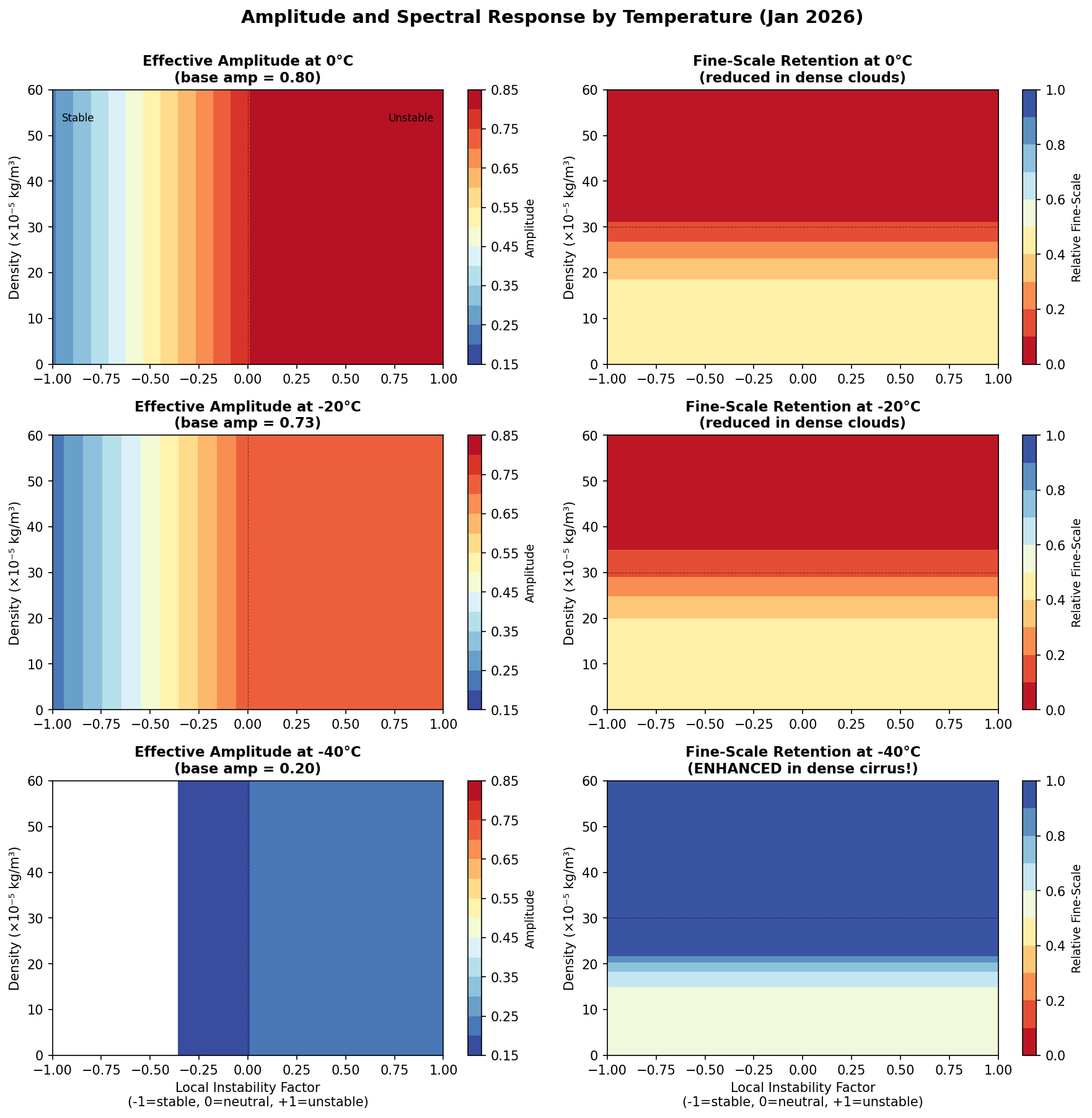
Figure 2: Three temperature slices (0°C, -20°C, -40°C) showing effective amplitude (left column) and fine-scale retention (right column). Key insight: fine-scale behavior reverses with temperature—warm clouds have fine scales REDUCED in dense areas (scattering physics), while cold cirrus has fine scales ENHANCED in dense areas (ice crystal optical properties favor sharper edges). The -20°C row shows transitional behavior.
Figure 3: Texture Magnitude Response
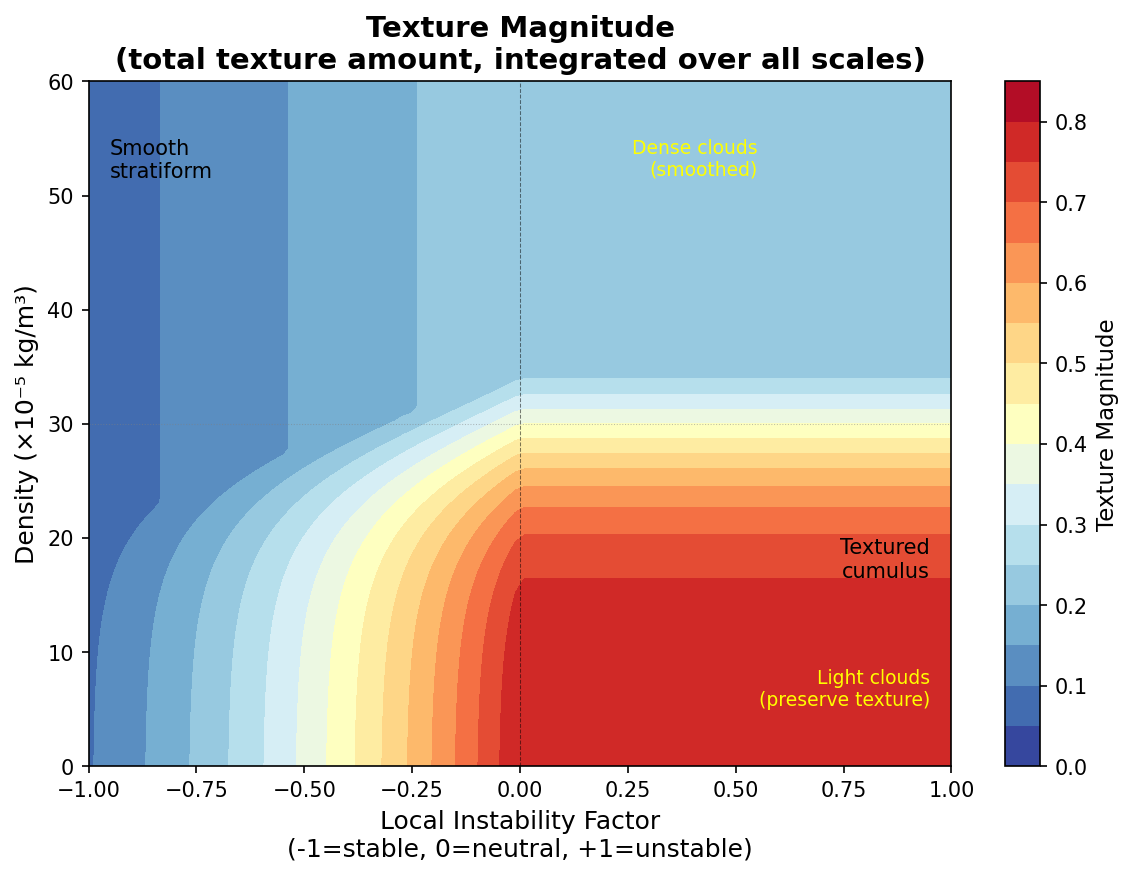
Figure 3: Total texture magnitude integrated over all scales. Shows how much texture survives stability and density effects, but not the spectral distribution (shown in Figure 2 Fine-Scale Retention panels). Assumes warm cloud conditions (0°C); conceptual visualization (amplitude × (1 - smoothing)).
Figure 4: Scale-Dependent Amplitude with Cirrus Reversal
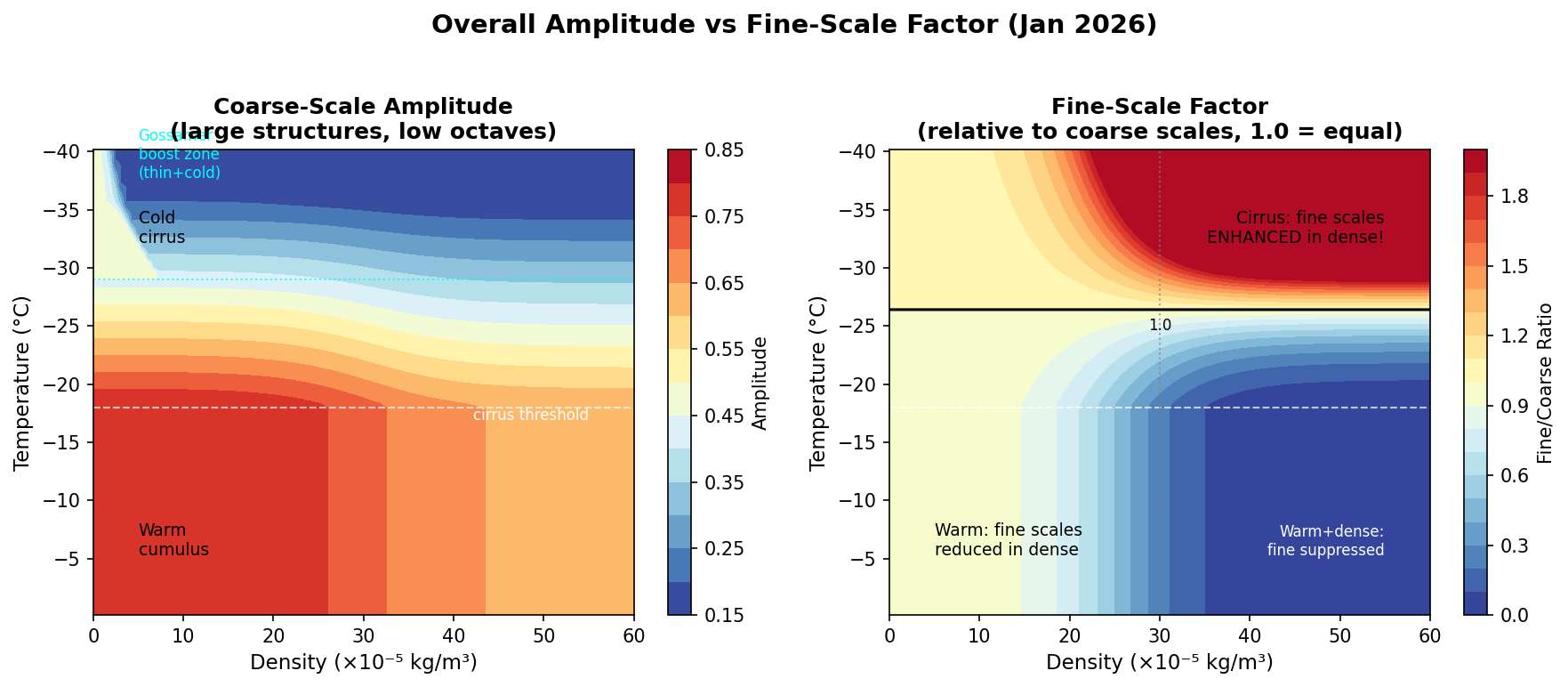
Figure 4: Left: Coarse-scale amplitude varies primarily with temperature, with slight density reduction. Right: Fine-scale amplitude shows temperature-dependent reversal—warm dense clouds have suppressed fine scales (smoother appearance), while cold dense cirrus has ENHANCED fine scales (sharper ice crystal edges). This matches observed cloud physics where ice crystals produce more distinct boundaries than water droplets.
Figure 5: Cirrus Richardson Number Physics
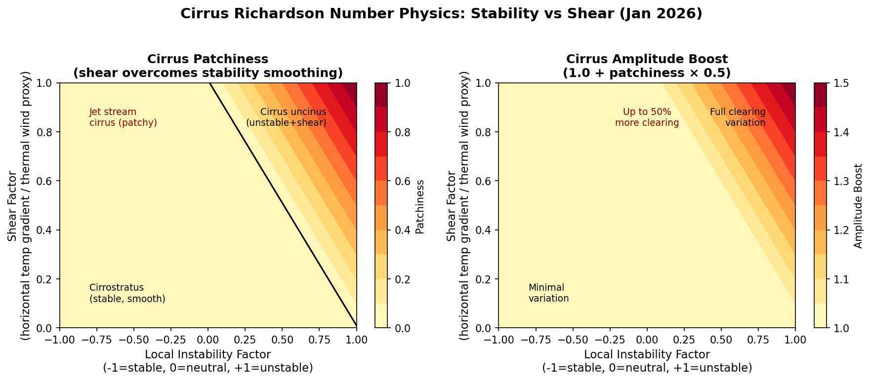
Figure 5: Richardson number-based patchiness for cirrus clouds. Left: Cirrus patchiness emerges when shear factor overcomes stability smoothing—jet stream cirrus (high shear, any stability) and cirrus uncinus (unstable + shear) show clear patches between generating heads at larger scales. Right: Amplitude boost up to 50% in patchy regions creates more pronounced clearings. Cirrostratus (stable, low shear) remains smooth.
3.5 Multi-Octave Noise Configuration
Both Perlin and Worley noise use a 6-octave fractal summation with cloud-type-dependent persistence to create appropriate texture at multiple scales.
Octave Parameters
- num_octaves: 6 (fixed for consistent multi-scale structure)
- lacunarity: 2.2 (scale ratio between octaves - slightly lower than 2.0 for smoother transitions)
- base_scale: Grid-relative, typically ~600-800m for coarse features
Persistence (Amplitude Decay)
- persistence_base: 0.80 (warm clouds)
- Cirrus adjustment: persistence = 0.80 + temp_factor × 0.15 → 0.80-0.95 range
- persistence_reduction_warm: 0.6 (strong fine-scale reduction for cumulus)
- persistence_reduction_cirrus: -1.0 (negative flips progression: fine octaves get MORE weight for wispy detail)
- Density modulation: Dense clouds reduce fine-scale persistence (scattering physics)
Perlin/Worley Blending Per Octave
- worley_weight: 0.0 (stable/cirrus) to 0.5 (warm+unstable cumulus)
- Blending formula:
octave_noise = (1 - worley_weight) × perlin + worley_weight × worley - Cumulus: Up to 50% Worley creates cellular convective structure
- Cirrus/Stratus: Pure Perlin for smooth layered appearance
Scale-Dependent Stretching
- Anisotropic stretching: Applied per-octave for cirrus streakiness
- scale_stretch_factor: Larger scales get more horizontal stretch
- vertical_correlation_factor: 2.0-8.0 range based on instability (taller cumulus turrets)
3.6 Additional Processing Components
- Ice Fraction Blending: Mixed-phase cloud processing blends liquid and ice water content with phase-appropriate physics
- 3D Volumetric Structure: Three-dimensional noise patterns create natural vertical coherence and clearing columns
- Constant Physics Weight: Uses physics_weight = 1.0 across all levels for pure Simplex behavior (bypasses level-dependent modulation)
3.7 Bypassed Legacy Systems
The following were bypassed to prevent level-dependent correlation issues:
- Atmospheric Seeding: Previously ±15% modulation based on temperature, pressure, humidity
- Cloud-Type-Specific Physics: CAPE integration, stability effects, wind shear patterns
- PDF-Based Enhancement: Probability density functions for cloud/clear distributions
- Complex Multi-Scale Systems: Multiple noise systems that broke vertical correlation
3.8 Thin Cirrus Gossamer Boost (January 2026)
Investigation of thin cold cirrus revealed that while anisotropic stretching (5:1) was correctly applied, the visual striations were invisible due to pattern amplitude being capped at 0.20. This enhancement boosts amplitude for thin cold cirrus to create visible gossamer texture.
Problem Analysis
- Observation: Thin cirrus at 233K showed no visible striations despite correct 5:1 anisotropic stretch
- Root cause:
pattern_amplitudecapped at 0.20 for cold cirrus (temp_factor ≈ 1.0) - Anti-mottling ruled out: density_factor was low (0.11-0.20), so smoothing was minimal
- Comparison case: Visible striations in 262K altostratus had
pattern_amplitude = 0.80
Solution: Density-Aware Amplitude Boost
For cold cirrus (temp_factor > 0.5) with low density (density_factor < 0.3), boost the pattern amplitude:
Effect
- Trigger conditions: Cold (temp_factor > 0.5, i.e., T < 244K) AND thin (density_factor < 0.3)
- Boost magnitude: Up to 2.35× for very thin cirrus (density_factor ≈ 0)
- Example case: temp_factor=0.996, density_factor=0.15 → boost=1.68 → pattern_amplitude: 0.20 → 0.34
- Result: Visible gossamer texture with natural striation appearance
Spatial Structure Improvements
Camera comparison revealed the initial patterns were too "blobby" - lacking the fine, linear character of real cirrus striations. Two adjustments improve spatial structure:
- Increased stretch ratio: From 5:1 to 7:1 for cold cirrus (
stretch_ratio = 1.0 + temp_factor * 6.0) — more elongated, linear patterns - Reduced base scale: 30% reduction for cirrus (
base_scale_m * (1.0 - 0.3 * temp_factor)) — finer striations (490m vs 700m base scale) - Combined effect: Octave scales shift from 700→318→145→66→30m to ~490→223→101→46→21m for cold cirrus
Interaction with Existing Cirrus Mechanisms
- cirrus_amplitude_boost: Triggered by HIGH shear (jet stream) → amplifies pattern_value inside noise generator
- thin_cirrus_boost: Triggered by LOW density (thin clouds) → amplifies pattern_amplitude in parent routine
- Complementary: Thin cirrus near a jet stream gets BOTH boosts applied
- Gap filled: Thin cold cirrus in quiescent conditions (low shear) now gets visible texture
4. Ongoing and Potential Enhancements
4.1 Validation and Parameter Tuning
- SWIm/Camera Validation: Side-by-side comparison of Simulated Weather Imagery (SWIm) renderings vs. all-sky camera observations used throughout development to validate cloud structure and tune parameters (instability_factor, shear_factor, cirrus_amplitude_boost, density thresholds for modulation reduction, Perlin/Worley amplitudes over octaves)
- Statistical Metrics (future): Develop quantitative measures of pattern realism (power spectral density, spatial correlation)
- LES Benchmarking (future): Validate against Large Eddy Simulation results for pattern fidelity
- Domain Testing: Validate across different geographical regions, seasons, and meteorological regimes
4.2 Performance Optimization
- Automated Parameter Tuning: Use objective metrics (power spectral density, SSIM) to compare SWIm renderings with camera observations, enabling automated tuning of noise parameters across meteorological regimes
- Computational Efficiency: Optimize noise generation calls for large domains
- Memory Management: Streamline coordinate calculation and pattern storage
- GPU Acceleration: Investigate GPU-accelerated noise generation for larger domains
5. Methodological Approaches and Future Directions
5.1 Comparison of High-Resolution Cloud Modeling Methods
Several methodological approaches exist for generating high-resolution cloud fields, each with distinct characteristics suited to different applications:
Large Eddy Simulation (LES)
- Strengths: Highest physical fidelity, explicitly resolves turbulent eddies and cloud microphysics
- Limitations: Computationally intensive, primarily suited for research and offline analysis, typically focused on boundary layer clouds
- Training Data Value: LES output (e.g., MicroHH) provides valuable training data for ML approaches and validation benchmarks
Machine Learning / Camera-Based (e.g., Cloud4D)
- Strengths: Data-driven texture generation, high temporal resolution (5s), validated against ground-truth observations
- Approach: Cloud4D uses synchronized ground-based cameras with homography projection to reconstruct 3D cloud properties at 25m resolution
- Limitations: Requires training data, camera infrastructure, and QC systems; LES training data primarily covers boundary layer cumulus
- Reference: arxiv.org/html/2511.19431v2
Procedural Physics-Based (Current LAPS Approach)
- Strengths: Real-time operational capability, physics-interpretable, works with standard NWP fields, scalable to large domains
- Approach: Stability-aware Perlin/Worley blending at global coordinates—Worley cellular noise for warm unstable cumulus, Perlin for stratus/cirrus with anisotropic stretching
- Key Innovation: Lapse rate → stability_factor, temperature → warm_cloud_factor, product → effective_stability controls noise type and vertical turret structure
- Applications: Aviation weather, solar forecasting, emergency response, numerical weather prediction
- Generalization: Naturally extends to new regions and meteorological regimes without retraining
5.2 Future Direction: Camera-Informed Hybrid Approach
Inspired by Cloud4D methodology, a future enhancement combines all-sky camera observations with the existing satellite-derived 3D cloud analysis to achieve 50m resolution downscaling:
Conceptual Framework
- Satellite Analysis (500m): Provides 3D cloud structure (heights, LWP, cloud type) from multi-source fusion (NWP + visible/IR satellite + radar + METAR)
- All-Sky Camera: Provides high-resolution 2D texture that can be projected onto satellite-derived cloud heights via homography
- Key Insight: Unlike Cloud4D's multi-camera stereo for depth, the satellite analysis already provides 3D geometry—the camera adds fine-scale texture detail
Cloud-Type Stratification
- Boundary Layer Cumulus/Stratocumulus (0-3km): Camera-informed texture mapping where camera provides best detail
- Mid-level Clouds (3-5km): Hybrid approach with camera at larger scales
- Cirrus (5+ km): Retain procedural Perlin approach—LES training data for cirrus is limited, and physics-based anisotropy handles fall streaks well
Quality Control Requirements
- Pre-filtering: Sun/moon glare, lens artifacts, exposure saturation
- Spatial masking: Horizon obstructions, transients (birds, aircraft)
- Registration: 1-2km displacement correction for timing and navigation offsets
- Calibration: Geometric (lens), Radiometric (exposure), Temporal (sync), Spatial (registration)
Implementation Phases
- Phase 1: Procedural only (current—working)
- Phase 2: Add camera QC infrastructure, output diagnostics only
- Phase 3: Camera-informed low clouds with conservative QC
- Phase 4: Extend to mid/high levels with scale-appropriate weighting
Graceful Degradation
The system maintains robustness by falling back to procedural generation when camera data is unavailable or fails QC—ensuring output is never worse than the current operational approach.
6. Applications
- Numerical Weather Prediction: High-resolution cloud initialization
- Aviation Weather: Detailed cloud structure for flight planning
- Solar Energy: Fine-scale cloud forecasting for solar power prediction
- Climate Studies: Detailed cloud process representation
7. All-Sky Camera Case Studies
Side-by-side comparisons of SWIm (Simulated Weather Imagery) renderings with all-sky camera observations are used to validate cloud structure and tune algorithm parameters. These case studies document specific investigations and the resulting parameter adjustments.
7.1 Thin Cold Cirrus Gossamer Investigation (January 2026)
Case: allsky.log.260222235 — Thin cold cirrus at 233K (-40°C)
Initial Observation
- Problem: Linear striations not visible despite thin, cold cloud conditions
- Expected behavior: Gossamer wispy texture should be apparent
Diagnostic Log Analysis
| Parameter | Value | Interpretation |
|---|---|---|
| Temperature | 233.1K (-40°C) | Very cold, full cirrus regime |
| temp_factor | 0.996 | Maximum cirrus treatment |
| density_factor | 0.11-0.20 | Low — texture preserved (anti-mottling minimal) |
| h_aspect (stretch) | 4.98 | 5:1 anisotropic stretch IS applied correctly |
| pattern_amplitude | 0.180 | Capped at cirrus floor — BOTTLENECK |
| anti_mottle range | 0.78-0.91 | Only 13% variation — too subtle to see |
Comparison with Working Case
Reference: combined_260182200_v4.png — Visible striations in 262K altostratus
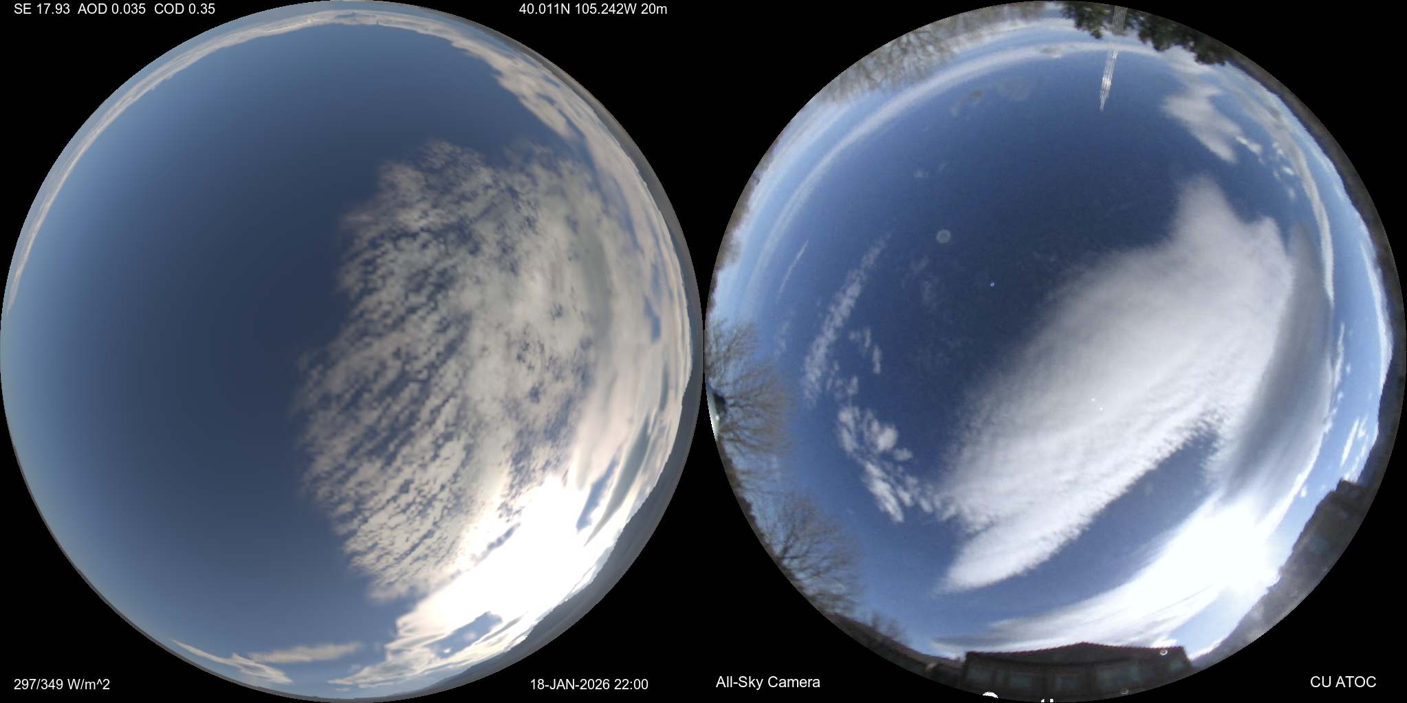
Figure 7.1: SWIm rendering (left) vs all-sky camera (right) — 262K altostratus showing visible texture variation with pattern_amplitude = 0.80
| Metric | Bad Case (233K cirrus) | Good Case (262K altostratus) |
|---|---|---|
| temp_factor | 0.996 | 0.0 |
| pattern_amplitude | 0.18 | 0.80 |
| anti_mottle range | 0.78-0.91 (13%) | 0.19-0.87 (68%) |
| Final output ratios | 1.7-2.1 (all enhancement) | 0.12-0.78 (real clearings) |
Root Cause & Resolution
- Root cause: The 0.20 pattern_amplitude floor (designed for subtle cirrus texture) was too restrictive for thin clouds where gossamer structure should be visible
- Not anti-mottling: density_factor was low enough that smoothing was minimal
- Resolution: Implemented
thin_cirrus_boost(Section 3.8) — boosts amplitude for cold + thin cirrus by up to 1.9× - Expected result: pattern_amplitude increased from 0.18 to ~0.26, creating visible gossamer texture