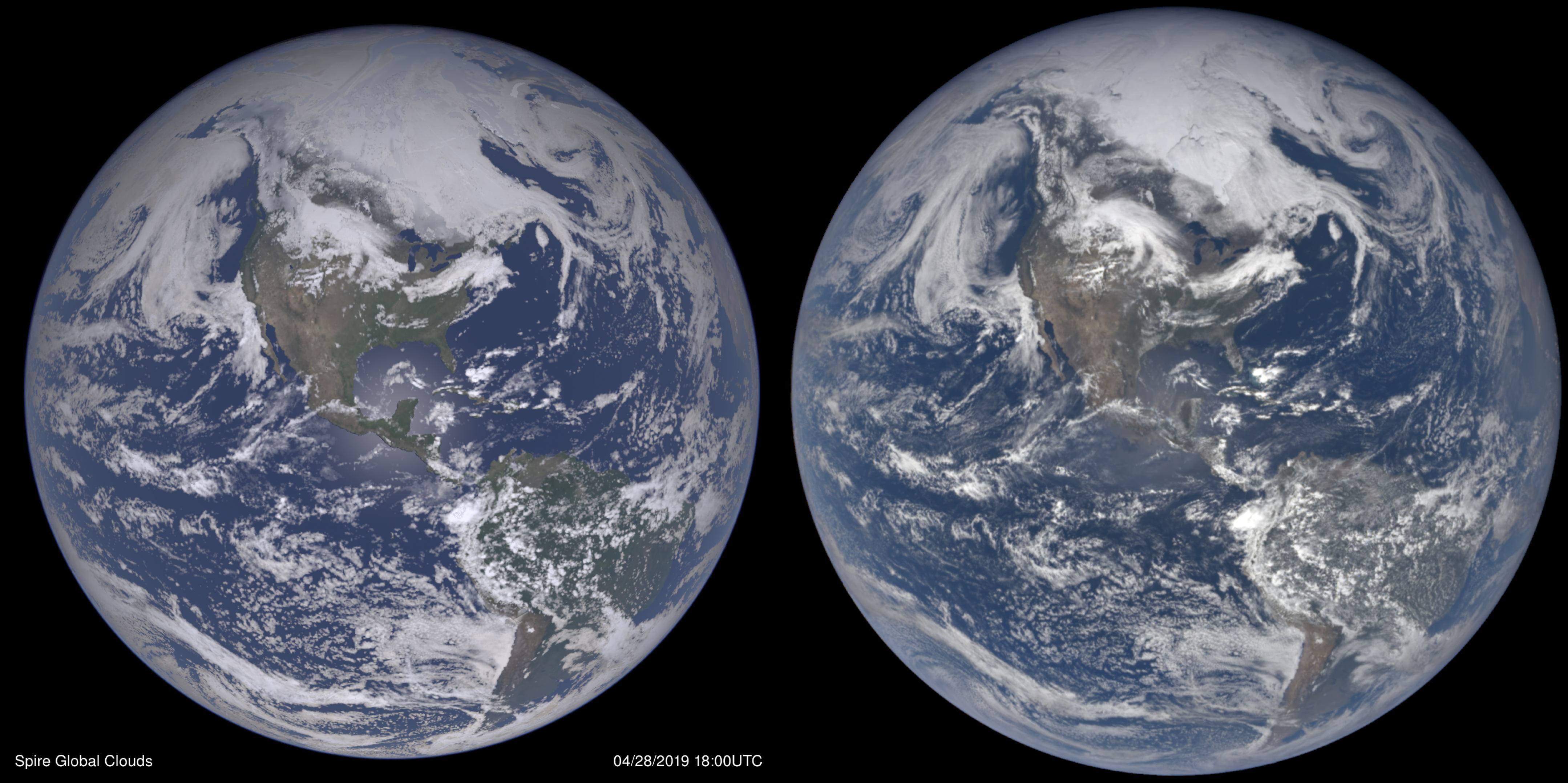
The image above on the left was synthesized using atmospheric data from a recent case that matches the actual DSCOVR image on the right, taken on April 28, 2019 at about 1800UTC.
I'm employing some fairly commonly used ray tracing (image rendering) techniques, with an emphasis on including the physical processes of visible radiation in the Earth's atmosphere and on the surface. Light rays from the sun and their associated photons can be considered to travel in straight lines, unless they are reflected or refracted. When encountering a cloud or the land surface the bouncing around of the light is called scattering. The angular pattern of scattering depends in interesting ways on the type of cloud or land surface, as well as the wavelength (color) of light.

Many or most light rays have a single scattering event and this is the easiest situation to calculate. The scattering occurs in partially random directions according to known phase functions (angular scattering probability distribution). However multiple scattering can get rather complicated as that can happen with several bounces in the atmosphere and even hundreds of times in a thick cloud. I've been working on ways to approximate multiple scattering as an equivalent single scattering event. This I hope will be providing a close enough result for many applications. There is another approach known as the Monte Carlo method that I may try eventually. Here we explicitly let individual photons bounce around in the scene, scattering in partially random directions according to the known phase functions. This is more computer intensive and even then some approximations are needed.
So what data do we need to run this simulation? NASA's Next Generation Blue Marble imagery provides high resolution color land surface information that can be approximately converted into spectral (color dependent) albedo. The conversion from the supplied image counts to albedo changes the brightness curve and helps give the land masses a more natural look. There are monthly versions of this to account for seasonal vegetation changes.
Key atmospheric gases are included such as nitrogen, oxygen, and ozone. The first two produce Rayleigh scattering and are mainly responsible for the blue sky. We see this blue sky both from the ground and from space. In fact the light we see over the oceans (outside of sun glint areas) is mostly atmospheric scattering and is the main reason the Blue Marble is blue. Thus the ground view of the blue overhead sky with thin scattered clouds (and the sun at a moderately low altitude) is rather similar (with a bit of imagination) to the space view looking straight down at the ocean! The blue cast is rather ubiquitous over both land and ocean and gradually increases in brightness as we approach the limb.
Ozone can produce a significant coloring effect when light travels at glancing angles through the stratosphere. Rather than scattering more blue light (like nitrogen and oxygen), ozone simply absorbs light. We might be more familiar with the ultraviolet absorption that protects us from things like sunburn. However there's also a lesser absorption in green and red light from the so-called Chappuis bands. Thus there's a blue window in its spectrum. From space a rising or setting sun can appear red when right near the Earth's limb (shining through the troposphere), though it can actually reverse color to be slightly blue when shining at a grazing angle through the ozone rich stratosphere. We can see a similar effect from the ground as a bluish edge to the Earth's shadow during a lunar eclipse. Ozone's coloring effects are almost imperceptible when looking up at the sky at midday, while during early twilight we see a blue overhead sky just as much from ozone absorption versus Rayleigh scattering. Thus there can be more to the familar question and answer to "Why is the sky blue?".
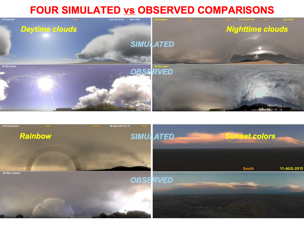
Clouds are of course a big part of the simulations and 3-D fields quantifying the density and size distributions of the constituent hydrometeors (cloud liquid, cloud ice, etc.) can be obtained from a Numerical Weather Prediction (NWP) model. In NWP, data assimilation procedures are used to combine weather satellite imagery, measured quasi-vertical profiles of temperature and humidity, surface and other observations and prior forecasts into 3-D analyses to describe the state of the atmosphere including clouds at any given time. In this case we're using a cloud analysis from an enhanced version of the Local Analysis and Prediction System (LAPS) that matches the time of the DSCOVR image. This system was selected because its cloud analysis is designed to closely match the locations of the actual clouds, particularly in the daylight hemisphere. The NWP analyses are also used to initialize NWP forecast models that project the initial state (including the clouds) into the future.
One aspect of evaluating the synthetic vs actual image match is whether the clouds lie in the correct locations. Another is whether they have the correct brightness, a sensitive indicator of the model's hydrometeors and the associated radiative transfer. All else being equal, optically thicker clouds are generally brighter as seen from above with more light scattered back toward space. This is the opposite of what we see when we're underneath a cloud. The cloud brightness or reflectance changes noticeably over a wide range of cloud thickness, allowing optical depth (tau) values from <1 up to several hundred to be discerned. This represents a wider range than can be distinguished with infrared wavelengths. Even when we're looking at a seemingly opaque cloud top we're actually learning about the properties throughout a great cloud depth. The cloud optical thickness in turn relates to the geometric thickness along with hydrometeor particle size and concentration. More details on the ray tracing algorithm can be found on our Simulated Weather Imagery (SWIm) page including a link to a powerpoint presentation based on a recent seminar.
Snow and ice cover on our planet can be compared, with the Antarctic ice sheets, sea ice, snow cover within Canadian forests as examples.
Sun glint is often visible in cloud-free regions over large bodies of water such as the oceans. The water roughness and wave slope statistics can be derived using a wave model that incorporates surface wind information. We can actually compare the sun-glint between SWIm and DSCOVR to see how well the winds and waves are being handled. Steeper waves will enlarge and/or dim the glint region. Calmer seas will cause the glint to brighten and contract. These effects apply to either the glint region as a whole, or to patchy regions within the glint envelope. Patchy dark areas in the glint often reflect localized calm winds. The glint can also change shape if it is significantly offset from the Earth's center. It can even change color to be more orange if there is heavy air pollution, or if the glint is near the limb of a crescent Earth - a different geometry than the nearly full Earth of DSCOVR's imagery.
Aerosols are here defined as particles other than clouds such as haze, dust, or smoke particles.
The ways to define aerosols are talked about in this
interesting blog post.
They are an important consideration and scatter light mostly in a forward direction.
They can be characterized by optical thickness (a measure of opacity), and scale height (indicating vertical distribution).
The sizes of the aerosols are typically in a bimodal distribution, where the larger dust particles scatter more light more tightly forward and smaller ones with a broader angular distribution.
Both aerosols and ozone help to soften the appearance of the Earth near the limb in the DSCOVR images, providing a sensitive test of the simulation.
Regional concentrations of aersols and their color can be compared,
such as air pollution surrounding India, and brownish dust blowing off of the Sahara into the Atlantic Ocean.
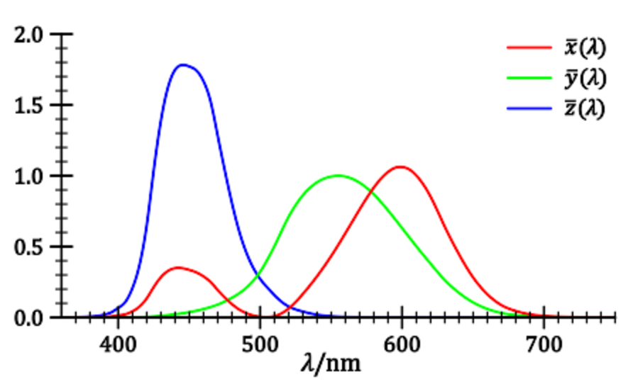
The ray-traced light intensities can be converted into the physical units of spectral radiance
by factoring in the solar spectrum. To convert the spectral radiance at each pixel location into an RGB color image
I take these steps to calculate what the image count values should be:
Background information about these three steps can be found here with an example for Rayleigh scattering.
An interesting aspect of the Rayleigh scattering example is that the blue Rayleigh sky is the same color as an incandescent object approaching infinite temperature, the values of xy are marked by the infinity sign along the Planckian locus of the chromaticity diagram. All incandescent light sources will have a color along this locus.
Both Rayleigh scattering and hot incandescent objects happen to follow similar inverse 4th power laws of radiance vs. wavelength.
A good example illustrating the benefits of the CIE color processing is in how the blue sky looks.
The violet component of the light is beyond what the blue phosphor can show, so a little bit of red light is mixed in.
This is analogous to what our eye-brain combination will do (for those with typical color vision). We thus perceive spectrally pure violet light in a manner similar to purple (a mix of blue with a little red).
While this is all a work in progress, I believe this should give a realistic color and brightness match
if you're sitting (floating) out in space holding your computer monitor side-by-side with the Earth.
This has somewhat more subtle colors and contrasts compared with many Earth images that we see. The intent here is to make
the displayed image have a proportional brightness to the actual scene without any
exaggeration in the color saturation (that is common even in everyday photography).
The presence of the atmosphere, more fully considered in the rendering helps soften the appearance of the underlying landscape.
Perhaps an astronaut can try these comparisons out sometime?
Going forward there's much here to learn about all the aspects of Earth modeling and raytracing improvements
to really demonstrate that we can model our planet in a holistic and accurate manner.
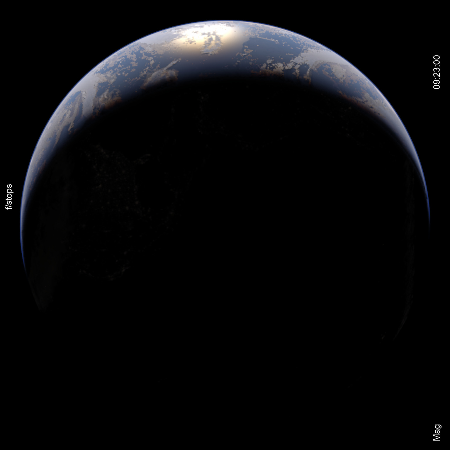
The DSCOVR satellite is positioned to always view the fully lit side of the Earth. The simulation package can also show us what DSCOVR would theoretically see
if it could magically observe from other phase angles.
Above is a simulated crescent Earth view from the same distance as DSCOVR.
Compare with an
actual image
from the Rosetta spacecraft as it flew by Earth.
Here is an animated version showing various phases that can be
compared with
this sequence
from the Himawari geosynchronous satellite.
Color Processing

Other Phases