This page describes the variational cloud / hydrometeor analysis and short-range nowcast running in real time in the LAPS 500 m Front Range domain, and sets out what it adds beyond a simple two-dimensional advection nowcast, together with its current limitations. Every number quoted below is measured on case studies, and each is named so the claims can be re-checked. Most of the testing so far covers leads to 20 minutes from the window start, the range of the real-time forecast; we are now extending the evaluation to 60-minute leads on archived cases, beginning with the 5 October case of section 5a.
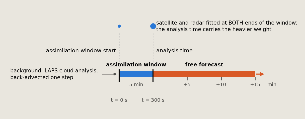
The analysis is a 4-D variational (4D-Var) fit of a cloud and hydrometeor field to satellite and radar observations over a short assimilation window. The window is 5 minutes and the analysis time is the window end, so the product is valid at the most recent observation rather than 5 minutes behind it.
Figure 1.1. The assimilation window: observations at each time are compared against the model state advected from one set of control variables at the window start, and the adjoint returns the gradient of the total cost with respect to those controls.
The control variable is the thermodynamic state at the window start on the full 3-D grid: liquid-water potential temperature θl and total water qt (the conserved pair), together with the vertical velocity w. Cloud liquid, cloud ice, vapour and temperature are not controlled directly; they are diagnosed from the pair by saturation adjustment, so condensate cannot exist without the water that makes it, and its latent heat is accounted for exactly. Rain, snow and graupel are taken from the background and carried through the model, and graupel contributes to the reflectivity operator. An earlier formulation controlled each hydrometeor species directly; several of the measurements in sections 3 to 6 were made with it, and they are dated so this is clear.
Writing x0 for that initial state and xb for the background, the cost function assembles four kinds of term:
     J(x0)  =  J_b(x0)                        background departure
             + SUM over obs times t of
                 w(t) * J_ir(t)               IR brightness temperature
               + w_vis(t) * J_vis(t)          visible reflectance factor
               + J_z(t)                       radar reflectivity, in Z-space
             + J_rh(x)                        humidity consistency
             + J_ph(x0)                       precipitation phase
Two distinct maps appear in the cost function, and it helps to keep them apart. The forward model propagates the state forward in time, from the window start to each observation time. The observation operator of section 2a then maps that state into observation space, rendering condensate as brightness temperature, reflectance factor and reflectivity. The adjoint runs back through both. The distinction is worth keeping: a model prognosticates, an operator evaluates. (In data-assimilation notation these are M and H respectively. Usage varies by field: the observation operator is sometimes termed a forward operator, particularly for radar, and remote-sensing work often calls it a forward model. On this page forward model always means the time propagation.)
Between observation times the conserved pair and the precipitation are carried by semi-Lagrangian advection on the effective wind field described in section 3a, sub-stepped to respect the Courant limit, and moved vertically by the analysed w. After each step the cloud, vapour and temperature are diagnosed again from the pair, so condensation and evaporation follow the motion. The trajectory weights are computed once and shared, so cloud and precipitation in the same air move together. The free forecast beyond the analysis time runs the same model, with its physics. Section 1e lists what is switched on in real time and the recommended presets (Table 1.2) and where each data source acts (Table 1.3), and section 2 sets out every process and its status.
The forward model, the radiative-transfer operators and the reflectivity operator are all written in MLX and differentiated by automatic differentiation on the Metal GPU. The adjoint is therefore exact with respect to the code that runs, so no separately maintained adjoint can drift out of step. The practical cost of this appears in section 2b: every process has to stay differentiable, ruling out hard threshold gates.
Minimization is by nonlinear conjugate gradient over nine iterations, arranged in three blocks, one for each control: θl, qt and w. Each block runs its own line search, because their gradient magnitudes differ by many orders of magnitude and a shared step length serves none of them. Within a block the step length is chosen region by region, from each 24 km region's own fit to the satellite (section 7c-i), and the cost function is compiled once per tile for speed. The domain is analysed in six overlapping tiles and the forecast runs once over the whole domain (section 7b).
The first guess is the LAPS cloud analysis for the window start, re-read every cycle; the analysis never starts from its own previous output. Before the control variables are built, a short sequence of steps corrects errors in that first guess which the minimization cannot correct by itself, because the observation gradient that would do it either vanishes or would act at the wrong height. Each step changes the background and the starting state together, so the background term does not pull the analysis back toward the uncorrected field. In the order they run:
The first guess takes its horizontal placement from the satellite but its vertical structure from the cloud analysis's assumption that the top is opaque, and that is where it is weakest: on the 5 October case, thin cirrus was missing aloft in 70–75% of the pixels where the water-vapour and window channels together place a thin top, and where present it sat about 200 hPa too low. Section 8c describes a planned first guess that takes its vertical structure from the background model's own columns instead.
The table gathers the real-time configuration in one place. Processes that are switched on but have no effect on this path are listed as such, so a switch is never mistaken for a process that is acting.
| Component | In real time |
|---|---|
| Controls | θl, qt and w at the window start; rain and snow from the background |
| Window | 5 minutes, two observation times; visible wherever the sun is more than 11° above the horizon at each pixel, rendered at that pixel's own sun angle, and infrared at both, radar reflectivity in Z-space, weighted so that the radar term is comparable to the satellite terms where there is echo |
| First-guess preparation | infrared trim, visible fit with observed motion, wave-cloud seed and balanced start, moisture staged at the wave ascent (RH 0.80), a moist halo (RH 0.80) around the fitted wave cloud, below-ground mask; layer repartition acts on about 3% of columns. Convective vertical motion comes from a parcel formed from the lowest levels above the ground and lifted from the top of that layer; it rises dry below its condensation level, stops once its buoyant energy is spent, and reaches no higher than the cloud top the infrared shows |
| Condensation and evaporation | on, by saturation adjustment of the pair with a subgrid ramp beginning at 85% relative humidity, in the window and the forecast |
| Latent heating of the air | on: temperature is diagnosed from the conserved pair, so condensation warms and evaporation cools |
| Vertical advection | on, vapour and condensate by the evolving w, with one anti-diffusive (MPDATA) correction under a non-oscillatory limiter (7 October), so no cell leaves the range of its vertical neighbours; nothing enters through the ground or the model top |
| Vertical motion | evolving, the same in the window and the forecast (9 October): a part anchored to the terrain and the standing wave, plus a convective part that is carried by the wind, relaxes toward the parcel ascent over 60 minutes, is projected onto mass continuity, and is capped at 3 m/s |
| Ice phase | the ice share of new condensate follows the current temperature, and ice is judged against ice saturation (5 October); cloud ice falls at a speed set by its content (9 October) |
| Sedimentation and autoconversion | on; cloud turns to precipitation above 0.5 g m-3, so low stratus does not drizzle where the radar sees no echo |
| Adiabatic lifting source, subsidence evaporation | switched on but bypassed: saturation adjustment already condenses rising air and evaporates sinking air, so they would count it twice |
| Accretion, precipitation evaporation | off |
| Winds | prescribed from the background model, blended toward the radar steering vector in precipitation cores (section 3a) and held fixed through the forecast; only the continuity projection adjusts them (8f) |
| Minimization | nine iterations, three blocks, regional step length chosen on the observation terms, which a block may take only when it does not worsen the fit to the observations (9 October), six tiles |
| Forecast | 15 minutes beyond the analysis time (20 minutes from the window start), same model and physics; archived cases are now also run to 60 minutes for evaluation |
Table 1.1. The real-time configuration as of 11 October 2026. "Bypassed" marks processes switched on whose effect the saturation adjustment already supplies.
Recommended combinations of settings. The analysis program has several hundred options, and the useful combinations are kept as named presets, selected with --preset. The configuration in Table 1.1 is the preset realtime: the real-time cycle runs it unchanged, adding only launch settings (tiling, logging and cadence). A test meant to match real time starts from --preset realtime and adds just the setting under test, so any difference in the result comes from that setting alone. Table 1.2 lists the presets and when to use each.
| Preset | What it is | Use it for |
|---|---|---|
| realtime recommended | The real-time configuration of Table 1.1: pair-standing plus the first-guess preparation, regional step length and physics safeguards added from 22 to 28 September 2026 | Every test that should match real time, and any rerun of an archived real-time case |
| pair-standing | The conserved pair (θl, qt) with w, the standing-wave seed and the lee-wave dipole; realtime is built on it, so a change here reaches real time as well | Comparisons with the conserved-pair line before the September additions |
| operational-zspace | The earlier species minimizer, with radar in Z-space | Reproducing results from before the conserved pair |
| operational, radar-zspace, radar-off | The July 2026 species-minimizer configurations, with and without radar | Reproducing July results |
| subset-quick | A small cloudy subset, in seconds | Quick checks while developing code |
Table 1.2. Presets: the recommended combinations of settings. Settings given explicitly on the command line take precedence over the preset, and each run prints the settings its preset supplied.
Where each data source acts. The observations enter the analysis at two stages. In the preparation of the first guess, each source places, trims or seeds the starting state directly. In the minimization, the analysis adjusts the conserved pair (θl, qt) and w so that the rendered observations match at both window times. The minimization is well suited to refining amount, height and small displacements, where the cost has a useful gradient. Creating cloud where the first guess has none, placing a standing wave, and removing condensate far from its observed position give the minimization little gradient to work with, so the preparation handles them. Table 1.3 shows how each source divides between the two stages.
| Source | Preparation of the first guess | Minimization |
|---|---|---|
| Background model (HRRR or NAM, via LGA) | temperature, humidity and winds for the window; rain and snow taken as they are; winds held fixed, blended toward the radar steering vector in precipitation cores | background term: the analysis stays close to the prepared first guess |
| LAPS cloud analysis | starting cloud field | cloud constraint at the end of the window |
| Infrared | removes first-guess cloud that renders too cold; sets the layer allowed for wave cloud; limits convective ascent to the cloud top the infrared shows | rendered brightness temperature fitted at both window times |
| Visible (by day) | fits the first guess column by column; the image sequence supplies the motion field; places and seeds the standing wave and its moist halo | rendered reflectance fitted at both window times |
| Radar | moisture lid from the echo top; steering winds in precipitation cores | reflectivity at both window times, with echo targets and an upper bound where the radar sees no echo, weighted to be comparable with the satellite terms where there is echo; rain and snow themselves are not controls in real time (8b) |
| Terrain | below-ground rules; terrain-forced vertical motion | below-ground rules in the model |
Table 1.3. How each data source divides between the preparation of the first guess and the minimization in the real-time configuration. The free forecast uses no observations; it carries the analysed state and vertical motion forward.
Cloud in the model moves with the wind at its own level. Every level is carried by the three-dimensional background wind, in the window and in the forecast, and precipitation cores are blended toward the radar steering vector (section 3a). Getting the motion right therefore means two things: moving cloud has to sit at the level whose wind moves as the cloud is seen to move, and standing wave cloud has to be held by standing lift while the air passes through it.
What the minimization contributes. The cost compares the rendered satellite and radar images at both ends of the window, and the model carries the state between them. The adjoint of that transport takes a misfit at the analysis time back along each level's own wind to the window start, so the minimization corrects amounts, edges and displacements of a few pixels in the natural 4D-Var way. The vertical motion is itself a control variable: seeded where the observed crests stand still, it is adjusted so that condensation on the ascent and evaporation on the descent keep each crest in place while the air flows through it (section 7a).
Moving cloud to a different level is harder for the minimization. In principle the same adjoint signal carries it: cloud at the wrong level ends the window displaced, and the misfit points to the level whose wind would have carried it correctly. In practice the signal is the wind difference between levels times five minutes, often a few kilometres and comparable to the visible footprint, and moving condensate to a new level means creating cloud in unsaturated air, where the gradient of the saturation adjustment vanishes. Measured on the moving high cloud, the minimization changes the share of condensate in each layer by at most two percentage points, and that small change is downward rather than toward the faster winds above.
So the height is chosen in the preparation of the first guess, in the terms the cost uses. The observed cloud motion is measured from the two visible images of the window (infrared at night) over the full domain, with a confidence for each column. Where the motion is confident and the cloud's present drift misses it by 3 m/s or more, the cloud is placed in a layer centred on the level whose wind matches the observed motion, kept within the range the infrared allows, and the humidity is set so the model keeps it there. This is the choice that minimizes the analysis-time visible misfit under advection, made directly rather than by following a gradient. Where the visible stays put over rugged terrain, the column is treated as standing wave cloud and receives standing lift instead. The minimization then refines amount, edges and small displacements around the height the preparation has set.
How well it works. In the real-time cycles since 26 September the height the analysis sees mostly agrees with the level whose wind matches the observed motion (section 7c-iii); on days of fast, extensive high cloud the harder limit is the wind, with no level matching the observed motion in up to two thirds of cloudy columns. On the optically thick high deck of 24 September the analysed cloud top, near 300 hPa, agrees with both the infrared (about 315 hPa) and the level whose wind matches the observed motion (275–300 hPa). What still slows that deck in the forecast is its depth, already present in the first guess: a third of its condensate lies below 400 hPa, where the wind is 5 to 7 m/s against the 12 m/s the tops show, and the visible sees deep enough into the deck to follow that slower cloud. A longer window, a control on each column's cloud height, or a term comparing the observed motion with the wind at the level the visible sees would let the minimization take on more of this itself.
The useful distinction here is diagnostic versus prognostic. Diagnostic physics takes the state as given and determines how it appears: the microphysical assumptions inside the observation operator, turning condensate into radiances and reflectivity. Prognostic physics evolves the state, creating, converting, moving and removing condensate over time. The diagnostic physics is active every cycle. Since the conserved pair went into real time, the core prognostic processes are active too: condensation and evaporation, latent heating, vertical transport, sedimentation, autoconversion and the fall of cloud ice, and since 9 October the vertical motion evolves through the window and the forecast. Growth processes for ice and graupel, and any feedback on the horizontal winds, remain absent. The three subsections below follow that split, Table 1.1 gathers what runs in real time, and section 7c-ii measures the physics against a physics-off run and simple image advection.
The phase reference is worth setting out in detail, since it governs both the humidity term of section 1a and the saturation quantities the operators depend on. Referenced to liquid at every temperature, a flat 70% relative-humidity threshold grows progressively more severe with height:
| Level | Temperature | 70% over liquid equals |
|---|---|---|
| 100 hPa | −71.7 °C | 133% over ice |
| 150 hPa | −63.3 °C | 126% over ice |
| 200 hPa | −50.1 °C | 113% over ice |
| 250 hPa | −38.5 °C | 102% over ice |
| 300 hPa | −29.5 °C | 93% over ice |
Table 2.1. Relative humidity over liquid that corresponds to ice saturation, by level. The 70% liquid threshold the older scheme used reaches 133% over ice at 100 hPa, which is why a single liquid-referenced threshold cannot serve the cold levels.
A liquid-referenced penalty therefore demands ice supersaturation at every cirrus level, and does so most strongly where it is least defensible, at the coldest levels where the weighting factor also grows. A second error compounds it: saturation specific humidity computed over liquid runs too large below freezing, so the condensate-to-saturation ratio that scales the penalty runs too small. Such a term is at once too strict in its threshold and too weak in its magnitude, leaving the weight parameter able only to trade one error against the other.
The correction blends saturation vapour pressure between the liquid and ice formulations using the same ice water fraction above, with the ice branch taken from the LAPS Goff–Gratch esice routine so that the analysis and the underlying cloud analysis agree by construction. Blending across a ramp rather than switching at 0 °C keeps the cost smooth, which prevents a kink that would stall the line search. The effective liquid-relative threshold then varies with temperature: about 70% near freezing, 59% at −40 °C, and 37% at −72 °C. Section 6 reports its measured effect.
Height inversion from observed cloud drift. Deployed 1 September 2026. On the current real-time configuration its gates keep about 3% of columns, mostly because of the terrain ceiling described below; the visible fit's use of observed motion (section 1d) now does most of this work. Infrared radiances constrain cloud-top temperature, and therefore height, far better than they constrain cloud amount, but the two trade off against each other: a cloud can be made to match an observed brightness temperature either by moving it or by thickening it, and the minimization has no strong preference. Observed cloud motion breaks that degeneracy from outside the radiance, because the speed and direction at which a cloud drifts identify the wind level it sits at.
The analysis therefore measures cloud drift by cross-correlation between successive visible images, compares it against the drift implied by the analysed cloud height, and where the two disagree redistributes condensate toward the level whose wind matches the observation. On the case it was developed for, this reduced the disagreement between observed and analysed cloud motion from 12.2 m/s to 1.5 m/s.
The redistribution is applied only where a stack of gates agrees that it is warranted, each gate stating a physical condition rather than a tuned threshold: the cloud must be optically thin, actually advecting, measurably misplaced, and the required motion must be achievable at some wind level in the column. All are smooth ramps rather than steps, because hard gates left visible discontinuities at their boundaries.
A terrain ceiling carries most of the benefit, and it is the one gate whose case is physical rather than empirical: cloud over high terrain is anchored orographic cloud, not advecting cirrus, and lifting it to a fast-wind level makes it advect away when it should stay put. Excluding columns above 2800 m improved the analysis figure of merit, preserved the motion gain, and halved the tail of forecast damage. Three earlier attempts to gate on cloud properties instead — observed brightness temperature, and target-level ice phase under two configurations — all failed the same way: with the other gates already keeping under 8% of columns, any further multiplicative ramp acts as a volume control rather than a discriminator. That is recorded here because it is a negative result worth not repeating.
The caveat is that terrain and regime are confounded in the single case this was established on, since the high terrain is also where that case's orographic cloud sat. A case with genuine mountain cirrus would separate "do not lift anchored orographic cloud" from "do not lift over mountains"; the second reading would suppress real cirrus over the Rockies. No such case is archived yet, and acquiring one is the highest-value outstanding item.
All of the following are implemented as elementwise operations so the adjoint flows through them, and each has its own switch. The real-time status of each is given in the second column, and summarised in Table 1.1.
| Process | Switch, and real-time status | Form | Note |
|---|---|---|---|
| Sedimentation | --precip-sink on (autoconversion is what feeds it) | 1-D upwind fall in z, sub-stepped for stability; rain 5 m/s, snow 1 m/s; mass past the lowest level leaves as surface precipitation | The module's own documentation calls this required for radar: rain at 5 m/s falls about six model levels in five minutes, so omitting it is a first-order error over the window |
| Vertical advection | --vertical-advect on, window and forecast | Vapour and condensate carried by the analysed vertical velocity in flux form, with one MPDATA anti-diffusive pass | The w it uses is a control variable, seeded from the observed wave crests where they stand still |
| Cloud condensation / evaporation | --sat-adjust, --fcst-condense on, window and forecast | Saturation adjustment of the conserved pair, with a subgrid ramp that begins condensing at 85% relative humidity. An older relaxation form remains for the species formulation | This is the sink that erodes a spreading anvil edge |
| Adiabatic lifting source | --lift-source, --k-lift on but bypassed by saturation adjustment | dqc/dt = −w ∂qsat/∂z for saturated ascent, applied as a direct source so it scales linearly with w | The linear form prevents saturation at small ascent rates, so stronger terrain-scale ascent produces proportionally more condensate |
| Subsidence evaporation | --oro-couplet, --oro-k-subs on but bypassed by saturation adjustment | Decay rate on existing condensate proportional to descent speed | The lee half of an orographic couplet. Without it the scheme adds cloud on a windward slope while leaving it downstream, so terrain cloud smears instead of staying anchored |
| Evolving vertical motion | --w-prog, --w-prog-continuity on, window and forecast | A convective part carried by the wind and relaxed toward the parcel ascent (60 min), projected onto mass continuity by an isobaric Poisson solve, added to a part anchored to terrain and standing waves | One routine serves the window and the forecast, so the analysis is fitted with the motion the forecast then uses |
| Cloud-ice fall | --ice-sediment on | Fall speed from the ice content (Heymsfield–Donner) | Removes ice that would otherwise only advect |
| Autoconversion | --precip-sink, --k-auto on | Cloud → precipitation above a content threshold, separate thresholds for liquid and ice | — |
| Accretion | --accrete, --k-accr off | Collection of cloud water by falling precipitation, Kessler-scaled | At a defensible rate it is statistically indistinguishable from being off |
| Precipitation evaporation / sublimation | --precip-evap off | Sink in subsaturated air, returning mass to vapour | The other missing leading-edge sink, on the precipitation side |
Table 2.2. Prognostic processes that are implemented and differentiable, with the switch for each, its real-time status and its form. "Bypassed" means switched on but superseded by the saturation adjustment.
Two cautions that the switch names do not convey. Condensation has two switches covering different intervals — one inside the assimilation window, one in the forecast that follows it — and enabling the wrong one leaves the interval of interest as pure advection. And a switch is only live if the term or process it feeds is on the path actually being run: the conserved-pair path bypasses the lifting source and subsidence evaporation, and each run prints a line for every such switch so a bypassed one is never mistaken for a tested one.
Section 8f describes the path from this kinematic forecast toward evolving dynamics.
The measurements in sections 3 to 6 were made in July and August 2026 with the earlier formulation that controlled each hydrometeor species directly, and with less physics in the forecast. The mechanisms they establish still apply; the numbers belong to that configuration. Section 7c-ii repeats the central comparison, against image advection, with the current one.
A single-layer 2-D advection nowcast moves everything at one speed. The atmosphere behaves otherwise. Measured on the case of 25 July 2026, 0050 UTC, the precipitating system and the cloud field move at speeds that differ by a factor of three:
| Field | Best-fit motion | Speed |
|---|---|---|
| Echo > 20 dBZ (15-min baseline) | +3.0 km E, −1.5 km N | 3.7 m/s |
| Convective cores > 35 dBZ | +2.5 km E, −1.5 km N | 3.2 m/s |
| IR cloud (anvil / cloud top) | +3.0 km E, −1.0 km N | 10.5 m/s |
Table 3.1. Best-fit motion of the reflectivity field against the cloud field over a 15-minute baseline. The two disagree in both speed and direction, which is what the hybrid advection of this section exists to represent.
Both are consistent with the wind profile: 250 hPa u = 15.2 m/s, 500–550 hPa 4.4–4.7 m/s, 700 hPa 0.7 m/s. The IR sees the anvil drifting with the upper winds while the precipitating system is steered by the mid levels.
Purely per-level 3-D advection fails for the opposite reason: under 19.6 m/s of shear it separates the echo levels by about 20 km in 15 minutes, tearing a storm apart vertically because nothing in a kinematic model holds it together. So the effective wind is a blend,
u_eff = u_3d + w(precip content) * (u_steer - u_3d)
where u_steer is a single deep-layer steering vector fitted from consecutive radar mosaics, and w ramps smoothly with local precipitation content. The result is 2-D coherent motion where a deep precipitating core should move as a unit, and the real 3-D winds in the anvil and in non-precipitating cloud, with a smooth transition so no artificial convergence is created at the storm edge. The blend engages on only about 2% of grid points, a deliberately narrow intervention.
Measured effect, 3-D reflectivity Equitable Threat Score at 20 dBZ, steered versus unsteered on the case of 25 July 2026, 0050 UTC:
| Lead | Unsteered | Steered | Change |
|---|---|---|---|
| +0 min (window end) | 0.6160 | 0.6160 | identical — clean control |
| +5 min | 0.4897 | 0.5289 | +8.0% |
| +10 min | 0.4010 | 0.4474 | +11.6% |
| +15 min | 0.3412 | 0.3917 | +14.8% |
Table 3.2. Forecast skill with and without the steering-wind blend, by lead. The window end is identical by construction and serves as the control that the comparison is clean.
The gain grows with lead, exactly as an accumulated displacement error should, and core-level (300–700 hPa) displacement spread tightens from 10.8 km to 3.8 km. On 28 July 2026 the vector was fitted from 22,299 echo points and reduced the mosaic-to-mosaic rms from 19.67 to 15.31 dBZ, a 22.2% improvement, before any forecast was run.
A 2-D advection nowcast can only move what it is given. The variational analysis can add what is missing. On 28 July 2026, 1800 UTC, the background carried far too little light echo; the increment supplied it, and the forecast then tracked the observations almost exactly. Column-maximum reflectivity, pixel counts:
| Valid | Observed ≥5 dBZ | 4D-Var | Model only (no increment) | Increment |
|---|---|---|---|---|
| 1755 (window start) | 56,419 | 51,208 | 33,930 | +17,278 |
| 1800 (analysis) | 60,459 | 38,825 | 29,755 | +9,070 |
| 1805 | 65,540 | 49,608 | 36,842 | +12,766 |
| 1810 | 69,011 | 61,187 | 45,789 | +15,398 |
| 1815 | 71,533 | 72,123 | 55,537 | +16,586 |
Table 3.3. Echo coverage above 5 dBZ at each window time: observed, analysed, and the model run without the increment. The difference between the last two is the information the assimilation supplies.
The "model only" column is the identical configuration run with the minimizer disabled, so the difference is the analysis increment and nothing else. It closes a genuine 22,000-pixel deficit against the observations, and the +20 minute forecast lands at 72,123 against 71,533 observed. That is information the observations carry, and assimilation is what delivers it.
The control is to run the same forecast model from the unassimilated cloud field, so that only the initial condition differs. That comparison run is called bgfcst, the background forecast. It is seeded from the LAPS cloud analysis at the analysis time and then shares everything else with the 4D-Var forecast: the same steering-blended winds, the same five-minute stepping, and the same physics path. Measured on 25 July 2026, 1800 UTC, over a domain-scale box, using a combined figure of merit (visible RMSE × 100 + IR RMSE), with both columns scored against the same observations at the same valid times:
| Lead | Valid | bgfcst | 4D-Var | Change |
|---|---|---|---|---|
| +0 (analysis) | 1800 | 7.55 | 6.56 | −13.1% — 4D-Var better |
| +5 min | 1805 | 12.93 | 9.65 | −25.4% — 4D-Var better |
| +10 min | 1810 | 15.17 | 12.93 | −14.8% — 4D-Var better |
| +15 min | 1815 | 17.35 | 15.59 | −10.1% — 4D-Var better |
Table 3.4. Forecast error against a run started from the unassimilated first guess, by lead. Negative change favours the assimilated start.
The two forecasts share one code path and differ only in their starting state: the same steering-blended winds, five-minute frames and condensation physics, and each lead stamped with its true valid time. That keeps the comparison controlled, so the difference is the assimilation and nothing else. The seeding switch that stamps the valid time correctly is off by default and has to be set for this comparison.
Section 2b lists the prognostic processes built into the model. The record below explains how each reached its present status in Table 1.1.
An important limitation applies to most of these tests: the analysis-time fit is a blunt instrument for them. A physically sound source or sink is absorbed by the minimizer: the analysis-time IR fit stayed flat at 6.84 K across a twenty-fold range of subsidence-evaporation rate, up to 97% decay per step, because the free condensate control compensated for the change the physics introduced. Only a pathological setting shows up at analysis time, and then only by breaking the fit outright. So a null result at the analysis time carries little diagnostic weight for these processes. They must be judged on the forecast, where the minimizer has finished and can absorb nothing. Several of the flat readings above were collected with the absorbing instrument, and the same redundancy is a large part of why the analysis and the forecast keep disagreeing about what helps.
The caution from section 5 still applies: the horizontal semi-Lagrangian scheme is not monotone, so rates tuned against it may partly compensate a numerical error.
One structural constraint shapes all of these: every process must be differentiable, because the adjoint is taken through the code that runs. Hard threshold gates have zero gradient below the knee, silently killing the adjoint wherever they bite, so the saturation and humidity gates are smooth ramps rather than clips, with the smoothing width set to zero recovering the original hard behaviour bit-for-bit. This is a real design cost of automatic differentiation, and it is why the rate constants above need re-derivation rather than direct adoption from a conventional microphysics scheme.
The forecast visibly grows a spreading anvil shield, and it grows it too fast: on 28 July 2026 the observed ≥5 dBZ area grew 27% in 20 minutes while the model grew 41%. The natural physical explanation is that an anvil spreading with no evaporation of cloud and no sedimentation of precipitation retains all its condensate at the leading edge. That explanation is correct as far as it goes, and at the time of this measurement those sinks were absent from the free forecast; both run in it now.
But a stronger and more fixable effect is also present, and it would be masked rather than cured by adding sinks. Running with the minimizer disabled, so the forecast is pure advection of a conserved scalar, total condensate still grows monotonically:
| Valid | Total condensate | Change per 5 min |
|---|---|---|
| 1755 | 249.22 | — |
| 1800 | 254.54 | +2.13% |
| 1805 | 261.46 | +2.72% |
| 1810 | 271.53 | +3.85% |
| 1815 | 282.89 | +4.18% |
Table 5.1. Total condensate through the forecast, showing the semi-Lagrangian scheme manufacturing mass. The per-interval change is positive under pure advection, where it should be zero.
Advection of a conserved scalar conserves its total mass, so the growth is numerical in origin: the semi-Lagrangian scheme uses a non-monotone cubic (Catmull-Rom) interpolation that overshoots at sharp gradients. Two diagnostics localize it:
So the overshoot has both a missing-sink component and a scheme component, and the order of work matters: a monotone or flux-conserving advection scheme should come before, or at least alongside, evaporation and sedimentation. Adding sinks first would tune them to cancel a numerical error, and would then be mis-tuned as soon as the scheme was fixed. A flux-form conservative scheme conserves exactly, though it costs roughly ten times as much, so the practical question is whether a monotonicity limiter on the existing interpolation recovers most of the benefit.
The source of the manufactured mass has since been measured. The cubic interpolation dips below zero on the clear side of every cloud edge, and those negative values are reset to zero, which adds material each step: on the 5 October case the negative part was 0.85% of the upper-level condensate per one-minute step, and pure advection of that case's anvil grew its mass 21% in 55 minutes. A per-level mass fixer removes that growth. A second effect remains with mass held fixed: repeated interpolation spreads cloud features one or two grid cells across, and the 5th-order, flux-form, positive-definite scheme WRF uses spreads them by the same amount, at ten times the cost. Tracking the cloud as particles keeps those features intact and conserves mass exactly, which makes a particle-in-cell scheme for condensate the candidate if this spreading turns out to matter.
The 5 October 2026 case (section 9) is a late-afternoon storm complex that was already decaying: its coldest tops were warming before the assimilation window, and its anvil shrank after about 20 minutes. It is the first case we have evaluated to 60 minutes, three times the real-time forecast range, and the problem described here only becomes large beyond 20 minutes. Our 60-minute forecast instead grew the area colder than −20 °C to more than three times the observed. The HRRR did the same from its own start, so on this case the excess is not ours alone, but the cause in our system could be traced step by step:
A first fix keeps humidity at no less than 90% of its first-guess value, and diagnoses the window-start cloud in visible-clear columns with the same sharp condensation the window integrates. The simulated water vapour then agrees with the satellite to about 2 K, the analysis needs about 40% less ascent in the storm region, and the 60-minute frequency bias for cloud colder than −20 °C is about 1.1, against more than 3 for the deployed forecast, with raw ETS close to the deployed system (Figure 5.1). Placement did not improve with it: at −20 °C the frequency-matched ETS is the same or slightly lower (Figure 5.2). It costs the coldest tops, below −40 °C, and on the other cases it trades a gain on the growth case against a loss of about 7% in the Boulder wave-cloud amplitude. A floor on humidity is also a rule, not an observation, which led to the work in section 5b.
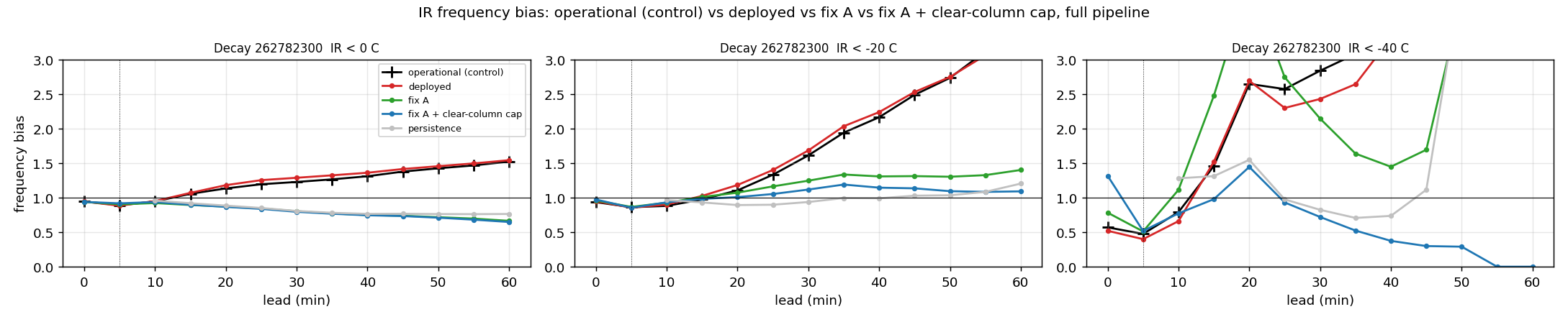
Figure 5.1. Infrared frequency bias by lead on the 5 October case at 0, −20 and −40 °C. The deployed forecast's −20 °C bias passes 3 by 55 minutes; with the humidity fix it stays near 1.1, close to persistence.
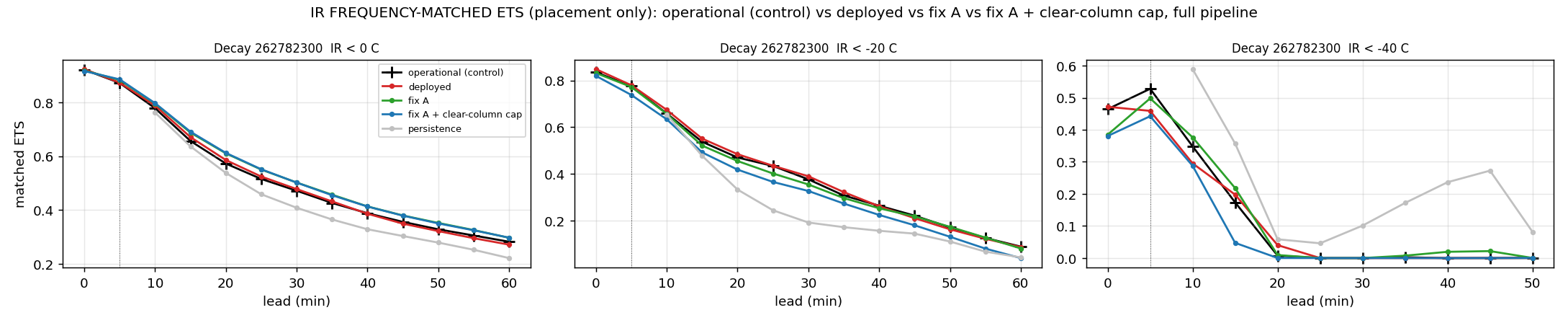
Figure 5.2. Frequency-matched infrared ETS by lead for the same runs: each forecast is thresholded at the brightness temperature that gives exactly the observed cloud area, so the score measures placement alone, independent of the amount shown in Figure 5.1. At 0 °C both humidity fixes place cloud slightly better than the deployed forecast from 15 minutes on. At −20 °C the floor alone tracks the deployed forecast and the floor with the clear-column cap is a little lower from 15 to 60 minutes, so the large improvement in amount comes without better placement of the cold cloud; at −40 °C the tops are lost after 15 minutes.
The water-vapour channel in the cost function. We added the GOES-19 6.9 µm channel to the infrared operator as a third channel of the same radiative transfer, with its vapour absorption varying with pressure, fitted to RTTOV 14: in clear air it reproduces RTTOV to 0.3–0.8 K and places its peak sensitivity within 0–25 hPa of RTTOV's. Against the satellite it removes the over-drying, from about +11 K to +1.6 K in clear air. But the minimization first met the observation with ascent, over about 70% of the domain at 300–400 hPa, and the forecast kept it: the 60-minute cold-cloud area grew more than fivefold. A constraint on large-scale vertical motion stopped that, and halved the 5 October bias, but it also removed the real mountain-scale vertical motion over the Front Range and cost the Boulder wave clouds. Used at the start of the window only, where it cannot reach the vertical motion, the channel corrects the humidity without harming the other cases.
A consistent state between stages. The window and the forecast had been starting from the background temperature while taking vapour and condensate from the analysis, so the liquid-water potential temperature they carried was not the analysed one. They now start from the analysed state in every field, which improves the forecast at most leads on five cases and removes the minimization's reliance on vertical motion to control the window's cloud. On the 5 October case the 60-minute excess remains, and section 4 lists the forecast-physics causes we now trace it to.
Section 2a sets out the correction itself. Its measurement is reported here in full, because the outcome differed from the expectation twice over: in the channel it acted through, and in its size. It also accounts for an earlier humidity-weight sweep where moderate values did nothing and a large value collapsed the upper-level cloud while degrading the IR fit by 7%, behaviour consistent with a mis-specified penalty applied hard.
The expectation was that this would work through the humidity penalty. The larger effect arrived instead through the observation operator, because the same relative humidity feeds the convective cloud-fraction diagnosis. Ice-aware humidity reads higher in cold air, so diagnosed cloud fraction rose:
| Domain | Mean diagnosed cloud fraction | Cells below 0.8 |
|---|---|---|
| Full domain | 0.82 → 0.94 | 44% → 6% |
| Cloudiest 200×200 subset | 0.60 → 0.87 | 100% → 20% |
Table 6.1. Diagnosed cloud fraction before and after the ice-phase saturation correction, with the count of cells below 0.8. The correction acts through the cloud-fraction channel rather than through the condensate directly.
This is a change in how a state renders rather than in the state itself, and the fields confirm it. Inside the analysed region the two configurations agree on condensate to within 0.3% (7.254 against 7.234, with 125,629 against 125,430 cloudy points, difference RMS 3.1×10⁻⁸) while their visible fits differ by 24%.
Using the combined figure of merit, ice-aware against liquid-only:
| Domain | Background | Analysis | Window start |
|---|---|---|---|
| Cloudiest 200×200 subset | −31.3% | −16.5% | −16.5% |
| Full domain | −7.6% | +0.9% | −3.8% |
Table 6.2. Size of the ice-phase correction on the full domain and on the cloudiest subset. The effect is domain-dependent, so the subset figure is not a general magnitude.
The subset promised a 16% improvement and the full domain returned about 1% the other way. Two effects account for the reversal, and both generalise beyond this correction:
Across the forecast leads on the full domain the ice-aware configuration runs about 1% behind at +5, +10, +15 and +20 minutes, with IR marginally ahead and visible marginally behind at every lead. On a separate daytime convective case the same isolated comparison came out roughly 0.7% ahead at analysis time. Two cases, comparable magnitude, opposite signs: the reading is that the combined score is indifferent to this change.
It stays in operational use for two reasons that survive that verdict. It is the physically correct formulation, and it removes a penalty that charged legitimate cirrus for existing. And it clearly improves the window-start fit, where the IR error moves from a 4% degradation to a 7% improvement, the end of the window that matters for getting the cloud evolution right.
One prediction from this work remains open. The corrected threshold should retain condensate near 125–175 hPa, where the air sits close to ice saturation, while thinning the ice-subsaturated levels at 100 hPa and 225–300 hPa. The stratiform test case produced almost no upper-level veil to begin with, 4 points against 1 above 200 hPa, so that test awaits a case carrying real cirrus. The 28 July 2026 case has 4,828 such points and is the intended vehicle.
This section records how the system running in real time came about, and what it measures. Its three parts are the handling of mountain wave cloud, which led to the conserved pair (7a); deploying that analysis over the full domain in tiles (7b); and the late-September work on the step length, the value of the physics, cloud height and the below-ground rule (7c). Table 1.1 summarises the resulting configuration. Problems still open at the end of this work are collected in section 8g.
How wave cloud is handled. The analysis treats cloud in two regimes. Everywhere by default, cloud is carried by the analysed wind: the conserved pair (total water and liquid-water potential temperature) is advected and the cloud species are diagnosed from it at every step. Standing wave cloud is added only where the observations show it, and only at the heights where it can exist:
Outside those columns and that layer nothing wave-specific is applied: cloud advects, and first-guess cloud that the infrared rejects is removed in the same way everywhere. The subsections give the evidence for the two regimes (7a-i), the change of variable they rest on (7a-ii), and the September 2026 work on height and on holding the crests in place (7a-iii). Deployment of this configuration is covered separately in 7b.
A case observed on 2 September 2026 at 1400 UTC turns the argument of 8f into a measurement. Mid-level cloud lay across the mountains, and the structure has two parts moving at different speeds: the wave crests are locked to the terrain while the cloud envelope advects through them. The forecast described in section 3a carries everything at one velocity, so it reproduces the envelope and carries the crests away with it.
Writing it as an equation makes the missing term explicit. What the observation requires is
dq/dt + U . grad(q) = S(x)
with S a source and sink fixed in space by the terrain, and its amplitude set by the
moisture the envelope delivers. Our forecast is the same expression with S = 0. The
two degenerate alternatives both fail: pure advection moves the crests, and holding the
field still would fix the crests but destroy the envelope, which we currently get right.
Scoring the forecast against persistence, on observed-cloudy pixels, separated into terrain relief terciles. Positive means the 4D-Var forecast is ahead; the table gives infrared RMS margin in kelvin against forecast lead:
| Case | Zone | analysis | +5 | +10 | +15 |
|---|---|---|---|---|---|
| 2 Sep, wave | high relief | +0.17 | −0.76 | −1.00 | −1.44 |
| flat | +2.44 | +2.49 | +3.38 | +3.19 | |
| 28 Jul, convective | high relief | +3.45 | — | — | +7.30 |
| 26 Jul, stratiform | high relief | +0.61 | — | — | +0.31 |
Table 7.1. Translation gain by terrain zone and lead for the two cases. Gain is the correlation at the best along-wind shift minus the correlation at zero shift; near-zero means the feature stands still.
Three things follow. On the wave case the forecast loses to persistence over high terrain and the gap widens with lead, while over flat ground in the same domain, at the same leads, it wins and its margin grows. The flat zone is the control: the model, the winds and the scheme are identical there, so this is not a general forecast failure but one tied to terrain. And the effect is not generic to mountains — on an ordinary convective case the forecast beats persistence over high relief by a growing margin, the opposite sign. The stratiform case sits between them. What distinguishes the wave case is that the terrain-locked part of the pattern carries enough of the variance to dominate the error.
A second signature points at the missing sink specifically. Splitting a ring around a Sawatch summit into upwind and lee halves by the observed flow direction, the forecast at +15 retains a 1.87 K advantage over persistence upwind and is level with it in the lee. Losing skill preferentially downstream is what a missing evaporation sink predicts, and no wind error produces that asymmetry. The samples are small — a few hundred pixels per half — so this is supporting evidence rather than a result on its own.
Cloud motion measured by cross-correlation returns 0.7 m/s in the visible and 2.2 m/s in the infrared where the analysed field moves at 8.8 m/s. That is not a failure of the measurement: on a stationary pattern multiplied by a moving envelope, a single cross-correlation returns a variance-weighted blend of the two. The consequence is that cloud-drift speed is not a velocity in this regime, and any inference that treats it as one — including the height inversion of section 2a — is inferring from a mixture. The speed gate rejects the slowest columns, but 22% of them pass it.
One approach was tried and does not work. Mapping cross-correlation speed against terrain to separate the crest and envelope components fails for a structural reason: a terrain-locked crest pattern is itself a stationary feature, so removing the static field to isolate moving cloud removes the crests along with it, and what remains is the envelope in both fields. Without that removal the correlation locks onto the land surface instead. The components do not separate by this route, and the terrain-relative error scoring above is what replaced it.
The separation does work, by scale rather than by speed against terrain (September 2026). Band-passing the two window-time visible fields into octaves and measuring the translation gain in each — the gain being the correlation at the best along-wind shift minus the correlation at zero shift — separates the two components cleanly on this case. The 4–8 km band, which is the crest scale, gains nothing from being shifted: its gain is −0.023. Every other scale gains, and the gains grow with scale: +0.039 at 2–4 km, +0.039 at 8–16 km and +0.057 at 16–32 km. So the crest band stands and everything both larger and smaller advects through it, which is the structure asserted at the head of this section, now measured directly from the observations with no model involved. Two cautions belong with that number. The raw gain is biased upward, since taking the best of twenty-one trial shifts finds some correlation in noise; the figures above subtract the same statistic computed across the wind, where advection cannot contribute, and the bias so measured runs from 0.000 to 0.023. And the position of the peak carries no quantitative meaning: calibrated against synthetic mixtures of a standing and an advecting field, the peak jumps from one component to the other rather than moving smoothly between them, so it ranks the two regimes without measuring their proportions.
The same measurement on a second case, 23 August 2026 at 1525 UTC, returns no standing band at all, the crest scale least of any: +0.108 at 4–8 km against +0.056 and +0.038 at the two scales above it. That case is a growth episode rather than a steady wave, and the contrast is what makes the first case's single standing scale meaningful rather than an artefact of the method.
The source term needs three things.
The wave structure is present. The forcing is a linear mountain-wave solution whose phase tilts with height, driven by a steering layer taken from 450–675 hPa, with a two-layer Scorer resonance and a closed-form trapped mode. It is not the boundary-layer upslope diagnostic that an in-phase terrain forcing would give. It reports a resonant wavelength of 10.1 km against 7–8 km observed. Two defects remain and both are measured. The amplitude is clipped: in the output field the vertical velocity reaches its ceiling at every level from 375 to 850 hPa and its ninetieth percentile sits exactly on that ceiling through 525–600 hPa, so the crests are flat-topped rather than sinusoidal. And the vertical decay is too weak: wave energy peaks at 575 hPa inside the steering layer, falls by roughly a factor of three by 300 hPa and then flattens near 1.2 m s-1 instead of decaying to zero, so a non-trapped residual reaches the tropopause.
Two defects of the earlier per-species formulation motivated the change of variable. Descent did not act as a sink: across the amplitude ladder the correlation between vertical motion and cloud change reached only −0.14, and the mean cloud change in descending air stayed positive at every lead. And condensate was placed without debiting the vapour that formed it: the small-scale total-water perturbation correlated with condensate at +0.32 to +0.39 through the wave-cloud layer, where a conserved formulation gives approximately zero. The remedy follows cloud-resolving models such as SAM (Khairoutdinov and Randall, 2003): analyse conserved quantities and diagnose vapour, liquid and ice from them, so that the inconsistency cannot be represented. The one constraint on what can be borrowed is that every operation must stay differentiable, so a smooth, analytically differentiable saturation adjustment is used in place of an iterative one. With the conserved pair in place, descent now does evaporate the crest cloud, losing 84–91% of it in five minutes (7a-iii).
The change of variable is implemented. Total water and liquid water potential temperature are now the analysed pair, with temperature, vapour, liquid and ice diagnosed from them, and the forward model advects the pair and re-diagnoses the species at every step rather than only at the initial time. The spatially fixed source S(x) that this section argues for is also built, as a vertical motion field placed from the observed visible imagery: its shape is the along-wind derivative of the observed cloud, which makes it zero-mean by construction and so balances ascent against descent, and its amplitude comes from the saturation inversion. On the wave case it improves the unassimilated ten-minute lead, taking the 4–8 km visible correlation from 0.401 to 0.438 and cloud-top correlation over cloudy pixels from 0.755 to 0.777.
What the configuration is worth, against the deployed analysis and against the cloud analysis it starts from. All three are archived for the wave case, so all three can be scored against the same observations over the same box with the same forward operator. The cloud analysis is included by re-running with the minimisation switched off, which leaves the analysis at its background, and with the seeding switched off so that background is the cloud analysis itself rather than a primed version of it. Root-mean-square error against the observations, infrared in kelvin and visible in reflectance, over the whole box and over the observed-cloudy pixels alone:
| Lead | Run | IR RMSE (K) | VIS RMSE (reflectance) | ||
|---|---|---|---|---|---|
| all | cloudy | all | cloudy | ||
| 0000 (1355Z) | LAPS cloud analysis | 1.763 | 2.100 | 0.0381 | 0.0791 |
| operational 4D-Var | 1.926 | 2.609 | 0.0430 | 0.0854 | |
| test 4D-Var | 1.741 | 2.188 | 0.0332 | 0.0487 | |
| 0005 (1400Z) | LAPS cloud analysis | 1.816 | 2.390 | 0.0404 | 0.0843 |
| operational 4D-Var | 1.628 | 2.854 | 0.0381 | 0.0794 | |
| test 4D-Var | 1.600 | 2.561 | 0.0279 | 0.0556 | |
Table 7.2. Error against the observations for the cloud analysis, the deployed 4D-Var and the test configuration, at both window times, over the whole box and over observed-cloudy pixels alone. Both leads are fitted times, so this is a fit diagnostic.
Three things are worth reading off this, and the second is not in the variational analysis's favour.
The test configuration has the lowest error in the visible at both times, by a wide margin over cloud — 0.0487 against 0.0791 for the cloud analysis at the window start, and 0.0556 against 0.0843 at the analysis time — and the lowest infrared error over the whole box. Against the deployed analysis it is ahead on all eight comparisons.
But both variational analyses are behind the cloud analysis in the infrared over cloudy pixels, at both times. The deployed one by 24% and 19%, the test one by 4% and 7%. The cloud analysis is built to match the infrared cloud-top signal directly and it does that better than either analysis that starts from it, so the variational step is currently trading cloud-top temperature for the visible structure it gains. The test configuration gives away far less of it than the deployed one does, which is the direction of travel, but it is a real cost and it belongs in Table 7.2 alongside the gains.
At the window start the deployed analysis is behind the cloud analysis on all four measures. That is defensible given the cost weights the end of the window more heavily than the start, so the window start is the end the deployed configuration has least reason to protect; it is recorded here rather than left out because it bears on how these numbers should be read.
Both leads are fitted times and the table is a fit diagnostic, not a forecast result. The analyses are drawn to the observations at 1355Z and 1400Z, and the conserved pair with a placed vertical motion has more freedom in its control vector than the deployed species analysis, so fitting those times more closely is partly what the extra freedom buys. What the table establishes is that the freedom is spent on the observations rather than against them. Whether it survives to times that were never fitted is the separate question answered at the unassimilated leads. The visible margin also has a mundane component: the visible term carries the larger weight at the analysis time, so it is the term the minimiser works hardest on. The cloudy masks hold 5,744 infrared and 26,121 visible pixels at the window start.
As an independent check, the cloud analysis reports its own fit in its logs, computed over the full domain with its own forward operator rather than the one used here: 2.539 K infrared and 0.0250 visible at 1355Z, and 2.622 K and 0.0263 at 1400Z. Those are not comparable line-for-line with the table — a different domain, mask and operator move the visible figure in particular by more than the margins being discussed — but they confirm the cloud analysis is performing normally on this case rather than unusually well or badly.
The case is archived with its verifying observations and its operational output. Nothing here rests on a single number, but all of it rests on a single case.
The 22 September 2026 case (section 9) combines lee-wave crests over Boulder County with a sky camera directly beneath them, which makes it possible to check cloud height as well as placement. Four findings shape the next step.
The remedy being tested is a balanced start confined to the wave-cloud region: the conserved temperature and total water are displaced along the streamlines implied by the seeded vertical motion, so that horizontal advection and lifting cancel and the crests stand still. Outside the wave region the fields are unchanged and cloud simply advects. A first version, balanced at the seeded points alone, drifted as before: its moistening left isolated moist patches that simply advected. Balanced over the whole wave zone, crests and troughs together, the drift over the window falls from about 1.5 km to 0.5 km, one grid point; the crests start on the observed ones, with a correlation of 0.76; and the visible misfit falls at both window times, by 74% at the start and 39% at the analysis time. A balanced start would also be a prerequisite for lengthening the assimilation window.
With the minimization, and over the full domain. On the Boulder subdomain the minimization keeps the balanced crests: the visible correlation rises from 0.73 to 0.75 at the start of the window and from 0.72 to 0.76 at the analysis time. Over the full domain, though, the wave zone spread to most of the grid, because every edge of visible cloud seeds it, and northwest Grand County, whose cloud advects, was brightened far past the observations. What separates the two regimes is visible directly in the imagery. Between the two visible images of the window the Boulder crests move about 1–2 m/s, within the noise of the image matching, while the northwest Grand County cloud moves 6–10 m/s east with the wind. Motion alone is not enough: a low deck over the flat southeast corner is just as still. The terrain supplies the second condition: the southeast deck lies over about 100–150 m of relief within 20 km, the Boulder crests over 600–1000 m. Requiring both, the balanced start is kept for about three quarters of the Boulder cloud, an eighth of the northwest Grand County cloud and none of the southeast deck. Elsewhere the staged moistening of the standing-wave seed continues as before.
Against the configuration it replaced in real time, this raised the Boulder visible correlation from 0.72 to 0.77 at the start of the window and from 0.73 to 0.80 at the analysis time, and the wave-band correlation from 0.72 to 0.81 at the analysis time. The combined infrared and visible figure of merit improved in every region at both times: over the full domain from 2.56 to 2.34 and from 3.41 to 2.79. The major Boulder wave clouds appear in the simulated visible image; some of the smaller crests are still missing, and the cloud cover at the analysis time remains under half of that observed. These results are from one case.
This concerns deploying the conserved-pair analysis as a whole rather than wave cloud specifically. The measurements below were made with eight tiles and twelve to twenty iterations; real time now runs six tiles, nine iterations and a regional step length (section 7c-i). Two of the three barriers to deployment have come down; the third has not.
Memory, which was the binding one, is resolved by tiling the analysis. The minimisation is the only phase that carries an adjoint tape — the forecast integrates without one — so only the analysis needs splitting, and its halo is set by how far information travels in one five-minute window rather than over a forecast. That distinction is worth about three times the overlap: roughly seven grid points of advection plus a five-point infrared footprint, against the thirty-four to sixty points a forecast-length cushion would demand. Tiling the 599×999 domain into eight pieces with a 24-point halo costs 23.6% extra work and peaks at 19 GB per tile against the 114 GB a single-piece analysis needs and the 20 GB the deployed system uses. One full-domain forecast then runs from the stitched analysis in 156 s at 20 GB, since it has no tape to hold. The complete cycle — eight tiles, stitch, forecast to +45 minutes — takes 22 minutes.
The analysis is better for being tiled, and the reason is physical rather than numerical. Several quantities the analysis treats as domain-wide are not uniform across it. The step normaliser is the largest gradient anywhere in the domain, and across a single 154×200 km box the two halves differ by a factor of 2.3, so every point in the weaker half is under-stepped by that factor. The steering wind varies 38% across the same box, and it sets both the amplitude of the inferred vertical motion, through the parcel transit time, and the direction of the dipole. Splitting the domain gives each region its own normaliser, its own line search and its own steering vector. Block-local normalisation recovers part of this without splitting anything, and it is now carried in the preset; the rest needs the split. Measured against a single tile that already has the block-local normaliser, on the wave case at 20 iterations with the error mask held 34 points inside the boundary:
| Lead | Run | IR RMSE (K) | VIS RMSE | VIS 9–14 km r |
|---|---|---|---|---|
| 0000, wave case | one tile | 1.841 | 0.0357 | 0.793 |
| eight tiles | 1.523 | 0.0329 | 0.853 | |
| 0005, wave case | one tile | 1.677 | 0.0314 | 0.918 |
| eight tiles | 1.666 | 0.0304 | 0.927 | |
| 0000, growth case | one tile | 3.206 | 0.0473 | 0.941 |
| eight tiles | 2.708 | 0.0442 | 0.948 | |
| 0005, growth case | one tile | 3.546 | 0.0580 | 0.898 |
| eight tiles | 3.292 | 0.0548 | 0.913 |
Table 7.3. Tiled against single-tile analysis at the two window times on both cases, with the error mask held 34 grid points inside the boundary. The single tile already carries the block-local step normaliser, so this isolates the split itself.
The line search bounds its step at one control scale. This prevents a few points in tile interiors from overshooting, which would otherwise degrade the infrared over cloudy pixels. A five-point ladder on both cases puts the best value at one: averaged over both cases and both window times it improves the infrared by 4.5%, the visible by 1.9% and the wave band by 1.6%, and at the window start it is the best of the five on seven of eight measures. With it, the tiled analysis is also better than the single tile over cloudy pixels at the window start, on both cases. One caution belongs with it: only the visible error at the window start varies monotonically with the bound. Everything else does not, because the bound changes which points the line search may move and so which solution it converges to, and a finer ladder would be measuring that rather than a trend.
Seams are a separate and smaller matter: the largest is a 0.24 K single-column step in temperature, and cross-fading the interiors over six grid points — free, since each tile already computes its halo — brings every seam below the typical column-to-column variation without measurably changing the scores. A fold of the cloud fields on the tile spacing shows no periodic imprint: fine-scale structure does run 16 to 35% higher within twelve points of a seam, but the untiled analysis shows a larger excess at the same columns, so that band is terrain and cloud rather than an artefact of splitting.
The iteration count is set by throughput rather than by the skill curve, and the shipping value carries a known cost. Measured end to end on both cases, the cycle takes 22.1 minutes of compute at twenty iterations and 16.0 at twelve. Against the single-tile reference across the sixteen window-lead measures, twenty iterations wins fifteen and twelve wins twelve; where twelve falls short it is the wave case at the analysis time, by 7.5% in the infrared and 13.9% over cloudy pixels. The preset carries twelve deliberately, the cheaper cycle having been preferred with that regression accepted and set aside for revisiting once more cases are available. Both configurations are archived and the choice is a single setting.
What sets the cycle time is contention, not the minimisation, which is why shortening the latter helps less than it appears. With the deployed five-minute cycle also running, the same work takes 31.5 minutes at twenty iterations and between 28.5 and 38.3 at twelve — the growth case at twelve took longer in wall clock than the wave case at twenty, on a third less compute. Per-tile times overlap almost entirely once queueing is counted, and the contention factor rises from about 1.45 to 1.78 as the compute shrinks, because fixed per-tile costs become a larger share. The levers that move the cadence are therefore standing the deployed cycle down while the tiled analysis runs, which gives 22 minutes, or an hourly update.
What remains is the radar term. It survives into the pair formulation but has almost nothing to act on, because rain and snow are taken from the background rather than carried in the control vector; switching radar off leaves the total-water and vertical-motion gradients unchanged to four significant figures. That was a loss of capability rather than a wiring detail. Since then the radar term has been weighted to parity with the satellite terms where there is echo (Table 1.1), and rain and snow can be carried as controls (8b).
Taken together over both cases, all four lead times and four measures, the configuration is better than a single tile on 26 of 32 comparisons and on 15 of the 16 at the two window times. The exception at the window times is cloudy-pixel infrared on the wave case at five minutes.
Three limitations belong with all of this. Everything above rests on two cases. The forecast leads are re-seeded from the written analysis rather than continuing in memory, which on the wave case costs about 10 to 13% of infrared error at ten and fifteen minutes while improving the visible by about 5% and the wave band by 3 to 5%; a control seeded from an untiled analysis through the same path loses the same amount, so the cost belongs to re-seeding rather than to splitting, and the growth case does not pay it at all. And the 22-minute cycle assumes the machine: with the five-minute deployed cycle also running, contention stretches it to 31.5 minutes, so a half-hourly update needs either a shorter minimisation, or the deployed cycle to stand aside on the half hour.
The real-time configuration changed several times in the last week of September. It now runs six tiles and nine iterations. The first guess is fitted to the visible image, with the observed cloud motion carried in the fit. The motion field is measured edge-aware, so the tile and domain edges leave no darker band behind. The cost is compiled once per tile, and the line search takes a separate step length for each region rather than one per tile. The subsections below cover the regional step, which made the larger tiles viable; compare the model against simple image advection and look at where the remaining error lies; and set out the rule that keeps hydrometeors above the ground.
A step length per region prevents larger tiles from losing skill. With a single step length for the whole tile, a region that wants a long step and one that wants a short step would have to compromise, and the more varied the cloud scenes within a tile, the more that compromise would cost. Choosing the step region by region removes that dependence on tile size, which lets the domain run in six tiles rather than eight and saves about 7% of compute.
The cost function now also returns its value column by column, split into an observation part and a background part, and the line search reduces those maps over 48-point regions (24 km). Each region then chooses its own step length from a parabola through its observation cost alone, and the step is accepted only where the total cost falls. Choosing from the observation part matters: the background part rewards small steps everywhere, and a region's fit to the satellite is what the step is meant to improve. The run checks that the column maps sum to the scalar cost.
| Case | Lead | 8 tiles, one step per tile | 6 tiles, regional step |
|---|---|---|---|
| Boulder lee waves | 0000 | 1.60 | 1.19 |
| 0005 | 2.46 | 2.22 | |
| Moving high cloud | 0000 | 2.03 | 1.53 |
| 0005 | 3.66 | 3.50 | |
| Orographic | 0000 | 3.31 | 2.92 |
| 0005 | 5.42 | 5.19 |
Table 7.4. Figure of merit, (IR RMSE / 2 K)² + (VIS RMSE / 0.03)², over the full domain at the two window times; lower is better. The regional step with fewer, larger tiles improves both window times on all three cases.
At night the regional-step configuration brought the infrared error on a night case from 6.08 to 3.89 K at the window start and from 6.28 to 5.38 K at the analysis time.
Which physics is active is listed in Table 1.1: condensation and evaporation through the conserved pair, latent heating, vertical transport, sedimentation and autoconversion, in the window and the forecast alike. The winds are prescribed, so there is no feedback on the flow and no pressure response, and ice growth, riming and melting are not represented (section 2c). This is partial physics: moist thermodynamics on a given flow, with no dynamics.
A fair test of what that physics contributes needs three forecasts rather than two. Image advection moves the observed satellite image along its own measured motion and is the standard no-physics nowcast. Our model with physics off runs the same analysis, minimization and three-dimensional winds, but between observation times it only advects, with no condensation, evaporation, vertical transport or sedimentation. Our model with physics on is the configuration above. Comparing the second and third isolates the physics; comparing the first and second isolates what the analysis and the three-dimensional winds add.
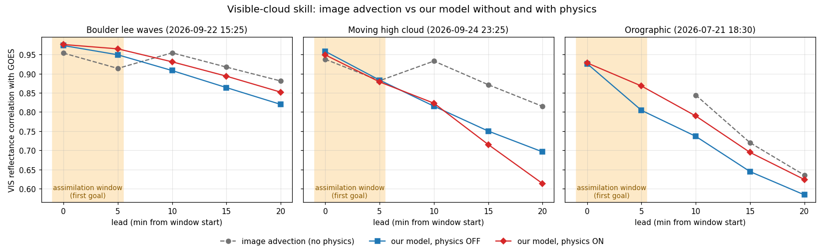
Figure 7.1. Visible correlation with GOES against lead. Shading marks the assimilation window. Image advection enters the free leads from the observed 0005 image, which is why its line jumps at lead 10. Both model forecasts use the real-time configuration of 28 September 2026 (Table 1.1).
| Case | Image advection | Physics off | Physics on |
|---|---|---|---|
| Boulder lee waves | 0.954 / 0.914 | 0.973 / 0.949 | 0.976 / 0.965 |
| Orographic | — | 0.926 / 0.804 | 0.928 / 0.868 |
| Moving high cloud | 0.938 / 0.882 | 0.958 / 0.883 | 0.949 / 0.879 |
Table 7.5. Visible correlation at the window start and the analysis time (0000 / 0005), real-time configuration of 28 September 2026. The orographic case has no image ten minutes before the window, so image advection cannot be formed there.
Within the window, where this system is meant to add value, the model beats image advection in visible correlation on both cases with a reference, and physics adds to it on the two terrain-driven cases. The one exception is the physics-on run for the high cloud, which falls just short of image advection in visible correlation while still having the lower infrared error and figure of merit (Figure 7.3). On the orographic case the physics raises the analysis-time correlation from 0.804 to 0.868, which is condensation and evaporation following the terrain-forced ascent and descent. On the moving high cloud the physics costs a little, since there is no terrain forcing and the diagnosed saturation adjustment changes a deck that should simply move. That cost has narrowed with the changes of late September (the moist halo, the parcel treatment of convective ascent and the closed lower boundary for vertical transport): from 0.014 and 0.022 at the two window times to 0.009 and 0.004, with the brightest high cloud closer to the observed brightness. The orographic gain at the analysis time is smaller than before, 0.064 against 0.079.
In the free forecast, image advection remains better on all three cases. It starts from the observed image at the analysis time, while the model starts from its own analysis, which fits that image to a correlation of 0.86 to 0.97 rather than exactly. The physics still helps the free forecast on the two terrain cases and hurts it on the high cloud beyond ten minutes, where the correlation at 20 minutes is 0.613 with physics against 0.696 without (0.584 against 0.694 before the late-September changes). On the Boulder case a wave crest brightens sharply between 15:25 and 15:30, just east of the main crests: the observed reflectance there goes from 0.103 to 0.200 and on to 0.240 at 15:35. Image advection moves these standing crests only about 0.3 km in five minutes, so it persists whichever image it starts from: 0.142 at 15:30, from the 15:20 image, and 0.199 at 15:35 only because it restarts from the observed 15:30 image, which already holds the crest. Our model follows the rise within the window, from 0.091 to 0.141 with physics on, while with it off the crest dims from 0.123 to 0.103; with physics on it reaches 0.220 at 15:35, the closest of the three to the observed 0.240.
The physics is also what keeps these crests in place. Tracking the analysed cloud itself, above ground only, the physics-off run carries it downwind at 8.3 m/s in the free forecast, the wind speed at 625–650 hPa and about 2.5 km every five minutes. With physics on the pattern does not move at all: air condenses where the standing lift raises it and evaporates where it sinks, so the crests re-form in place while the air blows through them. Within the window both move less than 2 m/s, because there the fit to the observed images holds the cloud. The physics-off panels of Figure 7.2 look steadier than this, because the simulated visible includes the fixed brightness of the ground, which dominates where the drifting cloud has thinned.
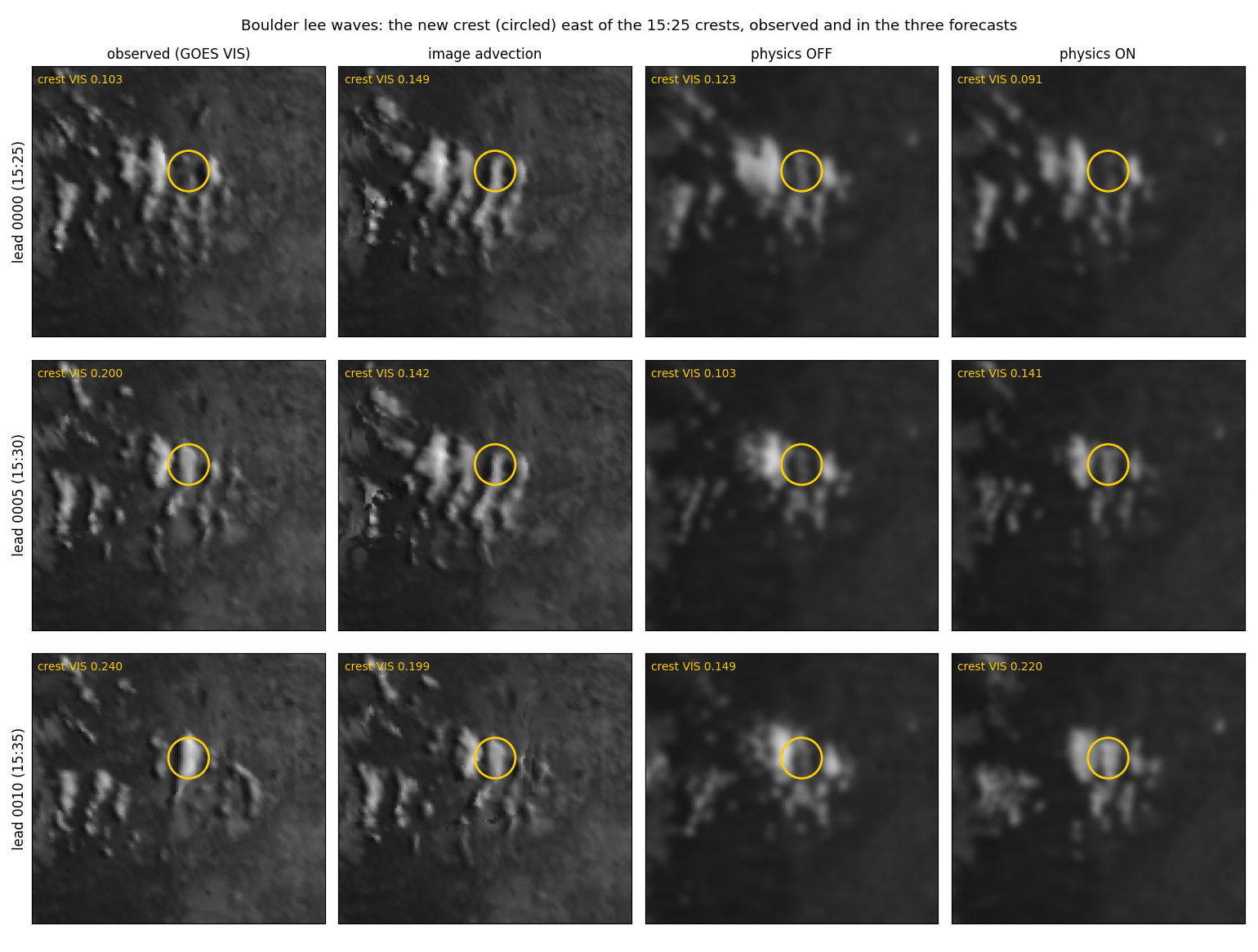
Figure 7.2. Boulder visible at 15:25, 15:30 and 15:35, observed and in the three forecasts, with the crest that brightens after 15:25 circled. Image advection barely moves these standing crests, so it persists its starting image.
The figure below adds the figure of merit and the infrared error for the same three forecasts. By the figure of merit, the physics improves the analysis on all three cases, including the moving high cloud, where its small visible cost is outweighed by a lower infrared error: at the analysis time the figure of merit falls from 3.49 to 2.19 on the Boulder case, from 4.28 to 3.15 on the high cloud and from 11.40 to 5.52 on the orographic case, and the infrared error from 2.43 to 1.86 K, 3.58 to 2.90 K and 4.70 to 2.98 K. The model with physics also beats image advection on both measures at both window times on the two cases with an image-advection reference. In the free forecast the physics keeps its lead throughout on the Boulder case; on the orographic case and the high cloud it leads at ten minutes, is level at fifteen, and falls behind at twenty, where the high cloud's infrared error is 7.9 K with physics against 6.9 K without. Image advection keeps its lead in the free forecast on every measure.
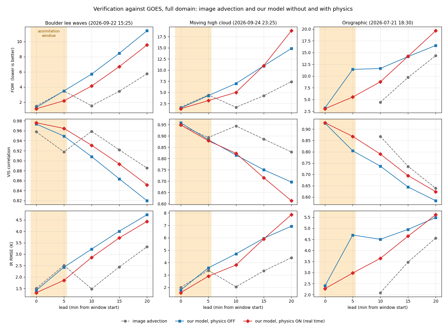
Figure 7.3. Full-domain figure of merit (top, lower is better), visible correlation (middle) and infrared RMSE (bottom) against lead, for image advection and the model with physics off and on (the real-time configuration of 28 September 2026).
Moving cloud belongs at the altitude whose wind carries it at its observed motion, and standing wave cloud at the height its infrared indicates. This section measures how far the analysis is from each.
Every real-time cycle is checked for this. For each cloudy column the background winds above ground are searched for the level whose motion matches the observed cloud motion, and that level is compared with the level the visible channel sees in the analysis, found from the operator's own two-stream contribution weights accumulated from the cloud top down. In the real-time cycles of 26 and 27 September the two agree to within 50 hPa, most often at the same level, and in most cycles the analysed level itself moves with the observed motion, within 3 m/s, in 55 to 80% of cloudy columns. Some level of the wind matches in 82 to 99% of them.
The first cases studied showed a larger gap, with the visible-weighted level 125 to 150 hPa below the matching one: 375 against 250 hPa for the high cloud of 24 September, and 725 against 575 hPa over the whole domain on the Boulder day. Cloud carried at the lower level moves with the slower, differently directed wind there, so its forecast drifts off the observed motion. For the optically thick high deck the difference is one of depth rather than of the top: its top, near 300 hPa, agrees with the infrared and with the level whose wind matches the observed motion, and the visible-weighted level sits lower because the visible sees deep into a deck whose lower third moves with slower winds (section 1f). On the orographic case the two levels agree, at 500 hPa.
On 28 and 29 September, with extensive, fast-moving high cloud, the analysed level lies at or up to 100 hPa above the matching one, and in 37 to 65% of cloudy columns no level of the background wind matches the observed motion within 3 m/s. There the limit is the wind, or cloud that develops rather than moves, and not the height. In the window the analysis leads image advection in visible correlation on each day scored, by 0.07 to 0.13 at the analysis time in the daily mean.
The infrared and visible channels see to different depths, which matters for how the height is inferred. Infrared is an emission measurement: absorption goes as exp(−τir) with τir about half the visible optical depth, so the infrared responds within the top visible τ of about 2. Visible reflectance comes from multiple scattering and saturates slowly, following the two-stream albedo bτ/(1 + bτ). With the backscatter fraction b of 0.15 for liquid and 0.19 for ice now used consistently in the operators, an albedo of one half falls at τ of 6 to 7, and the visible weights condensate nearly linearly below that. The aerosol backscatter uses 0.125, matching the LAPS cloud radiation module. The infrared footprint is also larger, so a small cloud partly filling it reads warm, and therefore low. This is why the footprint convolution in the operator matters. Correcting the infrared for the sub-footprint cloud fraction taken from the visible helps small features. It changes little for the thick high deck, whose optical depth near 27 fills the footprint.
Standing wave crests need a different test, since they do not move with the wind at any level. Here the infrared itself, corrected for how transparent thin cloud is, gives the height. The crests have a visible optical depth near 2 and an infrared emissivity near 0.5 to 0.6, so part of the warm ground shows through; solving for the cloud temperature that, at that emissivity, gives the observed brightness temperature places the tops about 2 km above the local terrain. Over the Continental Divide that is near 550 hPa, against the analysis at 625 hPa and 0.85 km above ground. Over the Boulder foothills it is 625–650 hPa, against the analysis at 700 hPa. The analysed wave cloud is therefore 50 to 75 hPa too low, and most so over the Divide, which is also how it looks from the sky camera.
Two attempts to raise it, on the Boulder subdomain, show what holds wave cloud in place. Placing the stationary wave cloud in the moist layer nearest each column's humidity maximum, between 700 and 450 hPa, overshot to 450–500 hPa and cost placement skill: the visible correlation at the window start fell from 0.86 to 0.75. The analysed standing vertical motion peaks at 625–650 hPa (0.4 to 0.8 m/s) and is under 0.1 m/s above 575 hPa, so cloud placed higher has no lift to hold it over the crests. It drifts downwind and evaporates within the window, because the fit leaves it as a thin saturated layer in air near 45% relative humidity that the advection's smoothing mixes away. Surrounding the fitted wave cloud with a moist halo, raised to 80% relative humidity and so still below the condensation threshold, keeps more of it alive. The halo reaches 1.5 km across and one level above and below the cloud, in stationary wave columns only, and never into columns the visible sees as clear; a wider 3 km reach left a faint veil in the simulated sky camera. Over the full domain it raises the Boulder wave-band correlation from 0.934 to 0.944 at the window start and from 0.788 to 0.851 at the analysis time, with the infrared error essentially unchanged (1.54 to 1.58 K). Over the Divide the share of visibly cloudy columns still holding cloud at the analysis time rises from 30 to 64%, and that cloud sits at 575 hPa, 1.6 km above the ground, against 625 hPa and 0.8 km without the halo: most of the way to the height the corrected infrared indicates. On the orographic case it is neutral. It has run in real time since 27 September 2026. Raising the cloud at the window start, which the visible fit still sets, is the remaining step.
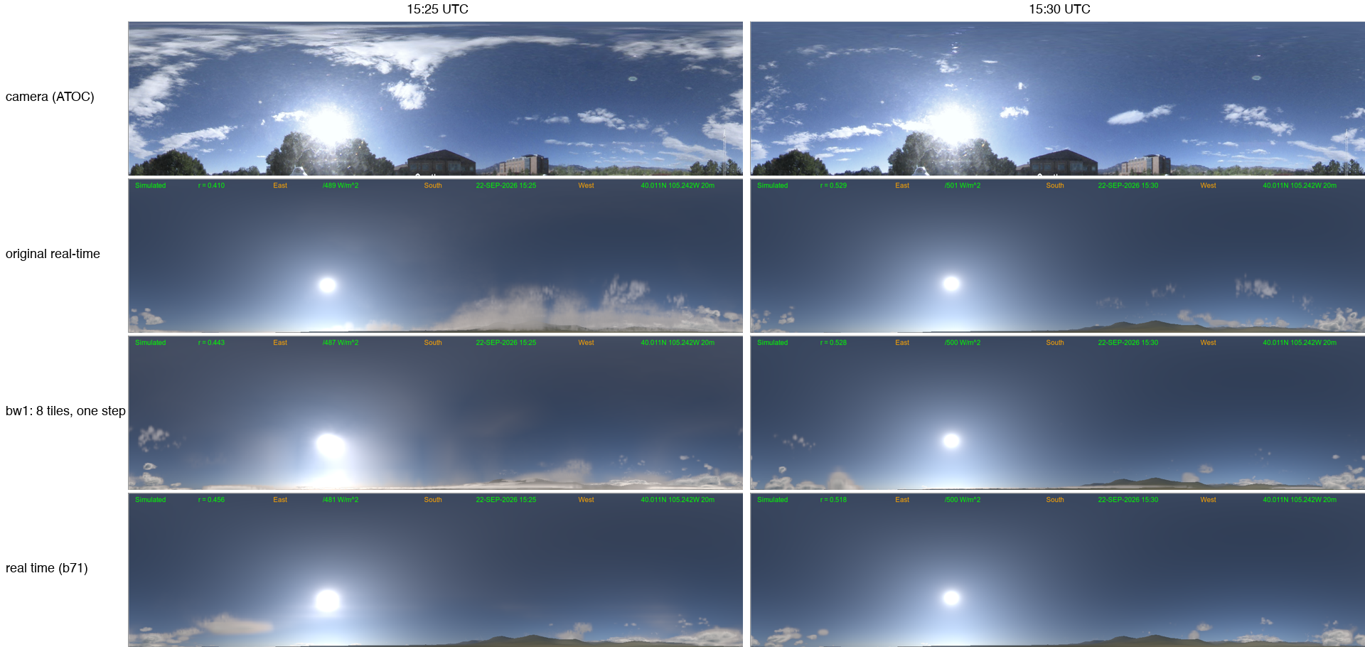
Figure 7.4. ATOC sky camera, Boulder, at 15:25 and 15:30 UTC, and simulated all-sky images from the original real-time analysis, the eight-tile rerun (bw1) and the real-time configuration of 28 September 2026 (b71). The r value printed on each simulated sky is its correlation with the camera image.
The sky camera shows both effects. The original real-time analysis put a false low deck across the southern and western sky. The real-time configuration removes it, and its sky correlates best with the camera at 15:25 (0.456, against 0.410 for the original and 0.443 for the eight-tile rerun); at 15:30 all three lie between 0.518 and 0.529. The wave cloud near the western horizon is present in all three simulations, but lower and less complete than in the camera.
Over the mountains the lower pressure levels of the grid continue beneath the ground. These underground points are fictitious, a numerical convenience with no real atmosphere and so no information about hydrometeors or humidity. A rule prevents spurious cloud from forming there, following the LAPS cloud analysis: cloud only above the terrain, precipitation down to the first pressure level below it. Underground water is kept as vapour, so total water is unchanged. The rule also keeps incorrect low cloud from developing in mountainous terrain, since cloud cannot form underground and then be carried up into the lowest levels above the ground (Figure 7.5).
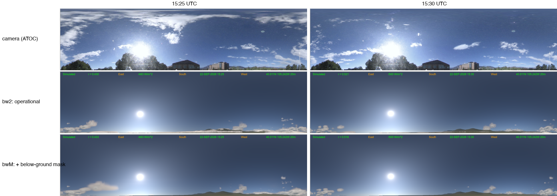
Figure 7.5. ATOC sky camera at 15:25 and 15:30 UTC, and simulated skies from the analysis without and with the below-ground rule. Without it, spurious low cloud lines the southern and western horizon at 15:25.
Monitoring. Every real-time cycle is now scored once its verifying images arrive. Each score is against GOES and against image advection over the same leads, together with the height check above. The results accumulate per domain, so the configuration is judged across many cycles rather than a handful of cases, alongside visual checks of the on-the-fly imagery.
Organised by component, following sections 1 to 3, so that each entry names the part of the algorithm it belongs to. Only the first is a strict prerequisite for the others.
This comes first, since section 5 shows the semi-Lagrangian scheme manufacturing condensate: a sink enabled before the scheme improves would be tuned against a numerical error, and mis-tuned as soon as the scheme was fixed. The cheap candidate is a monotonicity limiter on the existing cubic interpolation, clipping it to the local range of the donor stencil; a flux-form conservative scheme conserves exactly at roughly ten times the cost. The readout is simple: total condensate under a pure-advection run should stay flat.
Sedimentation, autoconversion, condensation and evaporation, and vertical transport now run in real time (Table 1.1), and the conserved pair supplies what the lifting source was meant to. What remains:
Beyond those, graupel generation and fall from section 2c are the leading candidate for the complete absence of core intensification described in section 4, since riming is what builds a convective core's reflectivity. Graupel currently advects as a passive tracer and appears in the reflectivity operator, with creation, removal and fall all still to be added. For convective cores this is the largest identified gap between the forecast and the observations; for wave and moving cloud it is cloud height (8g).
Most changes measured through August traded IR against visible; the September changes to the first guess and the per-pixel sun angle improve both. The visible residual is dominated by placement rather than amplitude, so height-aware cloud placement is the structural candidate for improving IR while keeping the visible gains. The warm IR bias drift with lead, present in both case studies, is the symptom to track. The phase reference corrected in section 2a also carries an untested prediction here: it should retain cirrus near 125–175 hPa while thinning the ice-subsaturated levels, and the 28 July 2026 case carries 4,828 suitable points to test it on.
Two refinements to the infrared term were added in September 2026. The second of them runs in real time; the first is off by default. The first corrects the liquid-cloud absorption at 11 µm. The operator had taken the absorption efficiency as one at every droplet size, which fixes the ratio of infrared to visible optical depth at one half. A Mie calculation for water at 11 µm gives an absorption efficiency of 0.84 at the 8 µm effective-radius floor and 0.71 at 6 µm, so thin small-droplet cloud, such as orographic wave cloud, is more transparent in the infrared, relative to its visible brightness, than the operator assumed: by 1.2 times at 8 µm and 1.4 times at 6 µm. A fit to the Mie result, accurate to about 1% from 4 to 30 µm, now replaces the fixed value when enabled. The second weights the infrared misfit more tightly wherever the simulated brightness temperature is colder than observed. Pixels whose observed temperature lies within 10 K of the surface are otherwise treated as clear and given a looser error, and that classification also covers warm low cloud, where a too-cold simulation indicates cloud the satellite does not see.
A first guess from the background model's columns. Our first guess has its placement from the satellite but its vertical structure from the opaque-top assumption (section 1d). A model background has the opposite strength: physically consistent vertical structure, but features in the wrong places. We plan to combine them by column matching, in the manner of database retrievals such as GPROF: for each observed pixel, take the vertical profiles of the background columns nearby whose simulated infrared, visible, water-vapour and split-window signals best match the observation. The database is whatever the LAPS background ingest provides in the lga, so it serves the HRRR here and another model elsewhere; the lga carries the background's cloud liquid, ice, rain, snow and precipitating ice. Because each column carries all of its layers, low and high clouds moving in different directions need no motion estimate. Candidate columns would come from similar terrain, and where no cloudy column lies nearby the cloud-analysis first guess remains. A related approach aligns the background's fields to the satellite with displacements estimated layer by layer, holding terrain-locked cloud in place. Both will be sized offline first, against the cloud-top heights retrieved from the water-vapour and window channels together.
A longer window. Two images five minutes apart cannot show whether a storm is growing or decaying. Earlier images, which we archive, would show that trend, and in sheared flow they do more: as the upper cloud slides over the lower, successive images expose different parts of the low cloud, which the window's level-by-level advection can then assemble.
All 16 channels. The real-time cost function fits two of the 16 ABI channels, the 0.64 µm visible and the 10.3 µm window, with the 6.9 µm water-vapour band and the 12.3 µm split-window band in testing (section 5b). The remaining bands carry information the analysis currently infers indirectly: the near-infrared bands (0.86, 1.6 and 2.2 µm) hold particle size and phase, 7.3 µm the mid-level humidity, 8.4 µm the phase again, and 13.3 µm the cloud height. Two published routes use all 16 channels (section 10): a retrieval of cloud-top products assimilated as a humidity proxy (Otsuka et al. 2021), and a learned mapping to water-content profiles on fine vertical layers (C3DIR, White et al. 2026). The plan here is to take the channels to the model levels directly: a C3DIR-style mapping as an engine for the first-guess vertical structure, and the cost function extended band by band, each new operator calibrated against RTTOV as the water-vapour band was. The infrared bands come first, being straightforward; the near-infrared reflectances need size-dependent operators, and 3.9 µm, mixing reflected sunlight with thermal emission, comes last. To our knowledge, direct assimilation of all 16 channels has yet to be attempted, so this extension would open new ground.
The step length is now chosen region by region (section 7c-i), which let the domain run in fewer, larger tiles and improves both window times on all three test cases. The conserved-pair formulation can add rain and snow blocks (8b); the rain block needs a smaller starting step than the others to descend. Choosing the step from each region's observation fit may also allow fewer iterations, shortening the cycle. Hakim et al. (2026; section 10) minimise a similar differentiable 4D-Var with AdamW, an adaptive per-element step suited to a cost surface as far from quadratic as ours. Adam directions fed into our line search descended more slowly, since the two then compete for control of the step; the test still to run is Adam in its own regime, as the step control over a fixed iteration budget.
Two measurement rules follow from what section 4a establishes. Physics is judged on the forecast rather than the analysis fit, since the minimizer absorbs a physically sound source or sink and an analysis-time null says little about it. And every substantive change is compared against simple image advection and against the same model with its physics off (section 7c-ii), while every real-time cycle is scored against both GOES and image advection as it verifies. Kurzrock et al. (2018; section 10) place the useful horizon of satellite cloud assimilation in hours, so as the window lengthens and the dynamics evolve (8f), the verification will extend from the present 60 minutes toward that range.
This remains a nowcast throughout. The target range stays at zero to a few hours, where observed structure still carries most of the skill, and adding dynamics leaves that unchanged. What changes is how much of the forecast advection has to carry on its own. Today it carries almost all of it, with a fitted steering vector standing in for storm motion.
The steering blend of section 3a is deliberately built to give way. Its weight reduces to zero to recover the real 3-D winds exactly, and it sits upstream of the advection routine, so improved dynamics modify the same wind field. Part of that path is now in place. The forecast carries cloud and moisture vertically, and takes its vertical motion from three diagnosed sources: terrain forcing, the standing lee-wave field placed by the analysis (7a), and convective ascent from a parcel buoyancy calculation capped at the infrared cloud top. The conserved θl–qt pair gives the latent heating of condensation and evaporation consistently. Since 9 October the convective part of the vertical motion also evolves, in the window and the forecast alike: it is carried by the wind, relaxes toward the parcel ascent of the current state, and is projected onto mass continuity, in the spirit of the pressure step of an anelastic model such as SAM.
What the established models have and this one lacks is momentum. WRF, the HRRR, SAM and ICON all carry the winds prognostically, so a storm's inflow and outflow respond to its heating and fade when it weakens, and rain-cooled downdrafts end it. Here the horizontal winds are held at their analysis values for the whole forecast, and section 5a shows the cost on a decaying storm. Three steps lead toward evolving winds, each taken only as far as it pays:
Advection then becomes one term among several rather than the whole forecast, and the prescribed storm motion can relax toward zero weight as the dynamics take the work over.
Kurzrock, F., S. Cros, F. Chane Ming, J. A. Otkin, A. Hutt, L. Linguet, G. Lajoie and R. Potthast, “A Review of the Use of Geostationary Satellite Observations in Regional-Scale Models for Short-term Cloud Forecasting”, Meteorologische Zeitschrift 27(4), 277–298 (2018). The review that frames this problem directly, and the closest survey of the family this system belongs to. Two points bear on the claims above: the field norm for the horizon over which satellite cloud assimilation demonstrably helps is measured in hours, against the 25–30 minutes quoted in section 4, so that horizon is a genuine weakness rather than a conservative statement; and the review identifies the treatment of vertical motion in cloud assimilation as an open gap, which is the gap section 7a addresses.
Satoh, M., B. Stevens, F. Judt, M. Khairoutdinov, S.-J. Lin, W. M. Putman and P. Düben, “Global Cloud-Resolving Models”, Current Climate Change Reports 5, 172–184 (2019), doi:10.1007/s40641-019-00131-0. Useful here for perspective rather than method. Global cloud-resolving models resolve nonhydrostatic motion at kilometre-scale meshes and abandon cumulus parameterization entirely, simulating cloud with explicit microphysics; the DYAMOND intercomparison it describes runs eight of them. They are solving a different problem from this one — global, free-running, and judged on convective and climate statistics over forty days, against a limited-area variational analysis judged on a sub-hour nowcast of a single orographic case. What transfers is the standard they set for the thermodynamics: at these scales the vapour/condensate partition is expected to follow from resolved dynamics and microphysics, not from an analysis increment placed by hand, which is precisely the defect identified in section 7a.
Khairoutdinov, M. F. and D. A. Randall, “Cloud Resolving Modeling of the ARM Summer 1997 IOP: Model Formulation, Results, Uncertainties, and Sensitivities”, Journal of the Atmospheric Sciences 60, 607–625 (2003) — the System for Atmospheric Modeling (SAM). The prior art for the change of variable proposed in section 7a: SAM advances liquid/ice water static energy together with total non-precipitating and total precipitating water, and diagnoses the vapour, liquid and ice split from those conserved quantities. The limit on what can be borrowed is that this system requires every operation to remain differentiable for the variational minimisation, so an iterative saturation adjustment is not directly usable.
Hakim, G. J., J. S. Whitaker, B. Huang and S. Frolov, “Long-window 4DVar for reanalysis using a differentiable weather model”, arXiv:2608.11515v1 (2026). The nearest published relative of the method used here: a variational analysis built on a differentiable model and minimised through automatic differentiation, with no separately maintained tangent linear and adjoint codes. Two of its choices bear directly on this system. It minimises with AdamW rather than conjugate gradient, on the argument that conjugate gradient assumes a quadratic cost surface and a nonlinear model does not provide one — a point that applies with force here, where saturation adjustment and the subgrid distribution switch condensation on and off and the total-water gradient carries a max/p90 ratio near 1200, and where the minimiser is still conjugate gradient. It also drops the background term altogether for windows of two to seven days, replacing it with a penalty on the first model step. That matters here because the same balance turns out to hold by accident rather than by design: measured on the conserved-pair configuration, the total-water background term sits around 10-8 of the total cost, so this analysis is already running with a background constraint that carries no weight, on a five-minute window. The distance is otherwise considerable — a global 2.8° reanalysis assimilating surface pressure alone over multi-day windows, against a limited-area cloud nowcast fitting satellite radiances over five minutes — so what transfers is the treatment of the optimisation, not the configuration.
Otsuka, M., H. Seko, M. Hayashi and K. Koizumi, “Data Validation and Mesoscale Assimilation of Himawari-8 Optimal Cloud Analysis Products”, Journal of Atmospheric and Oceanic Technology 38(2), 223–242 (2021), doi:10.1175/JTECH-D-20-0015.1. The first assimilation of cloud products derived from all 16 channels of a geostationary imager. The Himawari-8 optimal cloud analysis (an optimal-estimation retrieval with RTTOV, after Hayashi and Watts 2016) uses every channel of the Advanced Himawari Imager to retrieve cloud phase, top pressure, optical thickness and effective radius, with the visible, near-infrared and window channels each constraining one of these. The authors assimilate the result in JMA's mesoscale 4D-Var (JNoVA) as a pseudo-relative humidity: a cloud layer from the retrieved top down to a base estimated from the liquid water path at a fixed 0.3 g m-3, set to about 90% RH, and a climatological clear-sky value where the first guess is cloudy but the satellite sees none. Over two of three heavy-rain cases the 3-h rainfall threat scores improve, with the humidity increments driving wind changes through the 4D-Var tracer effect where low cloud traces inflow from the ocean. Three of their findings bear directly on this system. Their analysis kept the hydrometeors outside the control vector, since the retrieved water paths differed widely from the model's; here the condensate is analysed through the conserved pair and fitted to the radiances themselves. The retrieval describes the uppermost cloud layer, so low cloud beneath high cloud remains hidden to it; section 8c describes how successive images in a longer window can expose that cloud. And the vertical extent of the cloud is where the most is to be gained: the estimated base correlates at 0.30 with ceilometers, with an 890 m high bias, and the authors point to the statistical cloud-base method of Noh et al. (2017), used in the NOAA JPSS cloud products, and to variables closer to the cloud itself as the way forward. That is the direction taken here: to use the full channel set to map the satellite observations directly to the hydrometeors and water vapour at each model level, carrying the vertical structure that the channels hold into the analysis itself.
White, C. H., Y.-J. Noh, J. M. Haynes and I. Ebert-Uphoff, “C3DIR: A Deep Learning 3-Dimensional Cloud Property Retrieval Scheme for Passive Satellite Imagers”, arXiv:2607.16929 (2026), doi:10.48550/arXiv.2607.16929. A retrieval that draws on all 16 ABI channels (0.47–13.3 µm, pooled to a common 2 km grid), with the equivalent full channel sets of SEVIRI and AHI handled by the same network through a stem layer per instrument. Trained against EarthCARE cloud profiles matched along the imager's slant line of sight, and given a GFS short-range forecast of temperature and humidity, it returns vertical profiles of ice, cloud-liquid and rain water content on 0.25 km layers, together with cloud base, cloud top and multi-layer detection. The present system fits the 0.64 µm visible and 10.3 µm infrared bands, with the 6.9 µm water-vapour band (section 5b) and the 12.3 µm split-window band added in testing, each through its own forward operator inside the cost function. C3DIR shows how much vertical structure the full channel set carries, and its profiles are a natural candidate for the column-matching first guess of section 8c, where the vertical distribution of hydrometeors matters most: thin cloud aloft and cloud layered beneath it. Taken together, these two studies show the full channel set feeding a retrieval, and retrieved cloud products feeding an assimilation. Direct assimilation of the radiances themselves has so far covered the 0.6 µm visible band (operational at DWD since 2023) and the water-vapour and window infrared bands; to our knowledge, direct assimilation of all 16 channels has yet to be attempted. The present cost function already fits visible and several infrared bands together, making it a natural place to take that step.
All figures are single-case measurements unless stated otherwise. The combined figure of merit weights visible error roughly 2:1 against IR in practice. At +5, +10 and +15 the 4D-Var run is ahead in both channels separately, so those margins keep their sign under any reweighting. The analysis row does not: there the visible fit is marginally worse than the background's (by 0.004 reflectance) against a 1.40 K infrared gain, so a visible weighting more than about three times the present one would reverse that row alone.